

Assets

Llama 2: Efficient Fine-tuning Using Low-Rank Adaptation (LoRA) on Single GPU

Wed, 24 Apr 2024 14:23:28 -0000
|Read Time: 0 minutes
Introduction
With the growth in the parameter size and performance of large-language models (LLM), many users are increasingly interested in adapting them to their own use case with their own private dataset. These users can either search the market for an Enterprise-level application which is trained on large corpus of public datasets and might not be applicable to their internal use case or look into using the open-source pre-trained models and then fine-tuning them on their own proprietary data. Ensuring efficient resource utilization and cost-effectiveness are crucial when choosing a strategy for fine-tuning a large-language model, and the latter approach offers a more cost-effective and scalable solution given that it’s trained with known data and able to control the outcome of the model.
This blog investigates how Low-Rank Adaptation (LoRA) – a parameter effective fine-tuning technique – can be used to fine-tune Llama 2 7B model on single GPU. We were able to successfully fine-tune the Llama 2 7B model on a single Nvidia’s A100 40GB GPU and will provide a deep dive on how to configure the software environment to run the fine-tuning flow on Dell PowerEdge R760xa featuring NVIDIA A100 GPUs.
This work is in continuation to our previous work, where we performed an inferencing experiment on Llama2 7B and shared results on GPU performance during the process.
Memory bottleneck
When finetuning any LLM, it is important to understand the infrastructure needed to load and fine-tune the model. When we consider standard fine-tuning, where all the parameters are considered, it requires significant computational power to manage optimizer states and gradient checkpointing. The optimizer states and gradients usually result in a memory footprint which is approximately five times larger than the model itself. If we consider loading the model in fp16 (2 bytes per parameter), we will need around 84 GB of GPU memory, as shown in figure 1, which is not possible on a single A100-40 GB card. Hence, to overcome this memory capacity limitation on a single A100 GPU, we can use a parameter-efficient fine-tuning (PEFT) technique. We will be using one such technique known as Low-Rank Adaptation (LoRA) for this experiment.
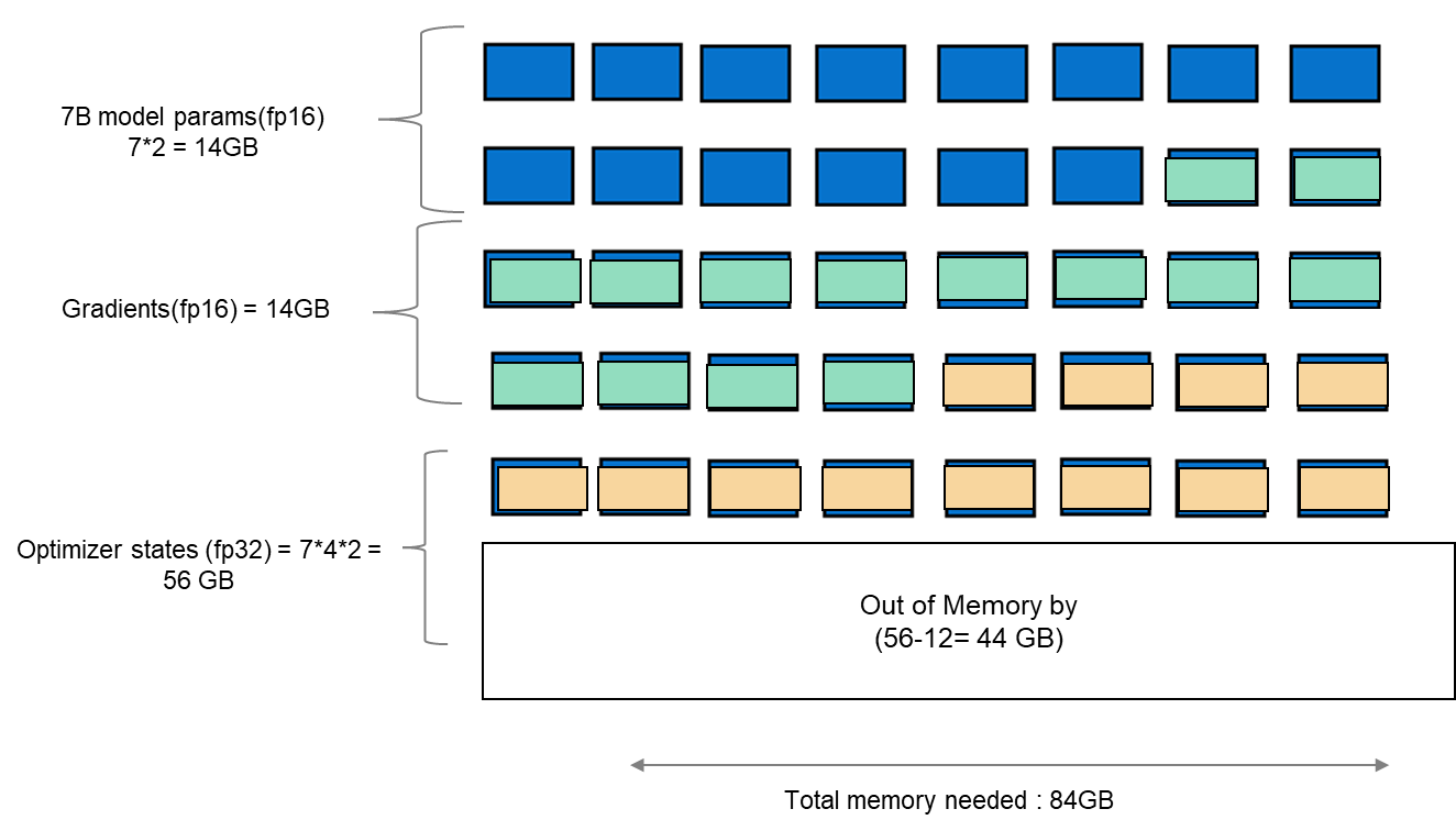
Figure 1. Schematic showing memory footprint of standard fine-tuning with Llama 27B model.
Fine-tuning method
LoRA is an efficient fine-tuning method where instead of finetuning all the weights that constitute the weight matrix of the pre-trained LLM, it optimizes rank decomposition matrices of the dense layers to change during adaptation. These matrices constitute the LoRA adapter. This fine-tuned adapter is then merged with the pre-trained model and used for inferencing. The number of parameters is determined by the rank and shape of the original weights. In practice, trainable parameters vary as low as 0.1% to 1% of all the parameters. As the number of parameters needing fine-tuning decreases, the size of gradients and optimizer states attached to them decrease accordingly. Thus, the overall size of the loaded model reduces. For example, the Llama 2 7B model parameters could be loaded in int8 (1 byte), with 1 GB trainable parameters loaded in fp16 (2 bytes). Hence, the size of the gradient (fp16), optimizer states (fp32), and activations (fp32) aggregates to approximately 7-9 GB. This brings the total size of the loaded model to be fine-tuned to 15-17 GB, as illustrated in figure 2.
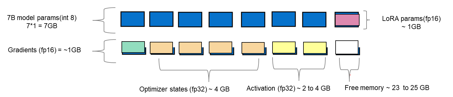
Figure 2. Schematic showing an example of memory footprint of LoRA fine tuning with Llama 2 7B model.
Experimental setup
A model characterization gives readers valuable insight into GPU memory utilization, training loss, and computational efficiency measured during fine-tuning by varying the batch size and observing out-of-memory (OOM) occurrence for a given dataset. In table 1, we show resource profiling when fine-tuning Llama 2 7B-chat model using LoRA technique on PowerEdge R760xa with 1*A100-40 GB on Open- source SAMsum dataset. To measure tera floating-point operations (TFLOPs) on the GPU, the DeepSpeed Flops Profiler was used. Table 1 gives the detail on the system used for this experiment.
Table 1. Actual memory footprint of Llama 27B model using LoRA technique in our experiment.
Trainable params (LoRA) | 0.0042 B (0.06% of 7B model) |
7B model params(int8) | 7 GB |
Lora adapter (fp16) | 0.0084 GB |
Gradients (fp32) | 0.0168 GB |
Optimizer States(fp32) | 0.0168 GB |
Activation | 2.96 GB |
Total memory for batch size 1 | 10 GB = 9.31 GiB |
System configuration
In this section, we list the hardware and software system configuration of the R760xa PowerEdge server used in this experiment for the fine-tuning work of Llama-2 7B model. 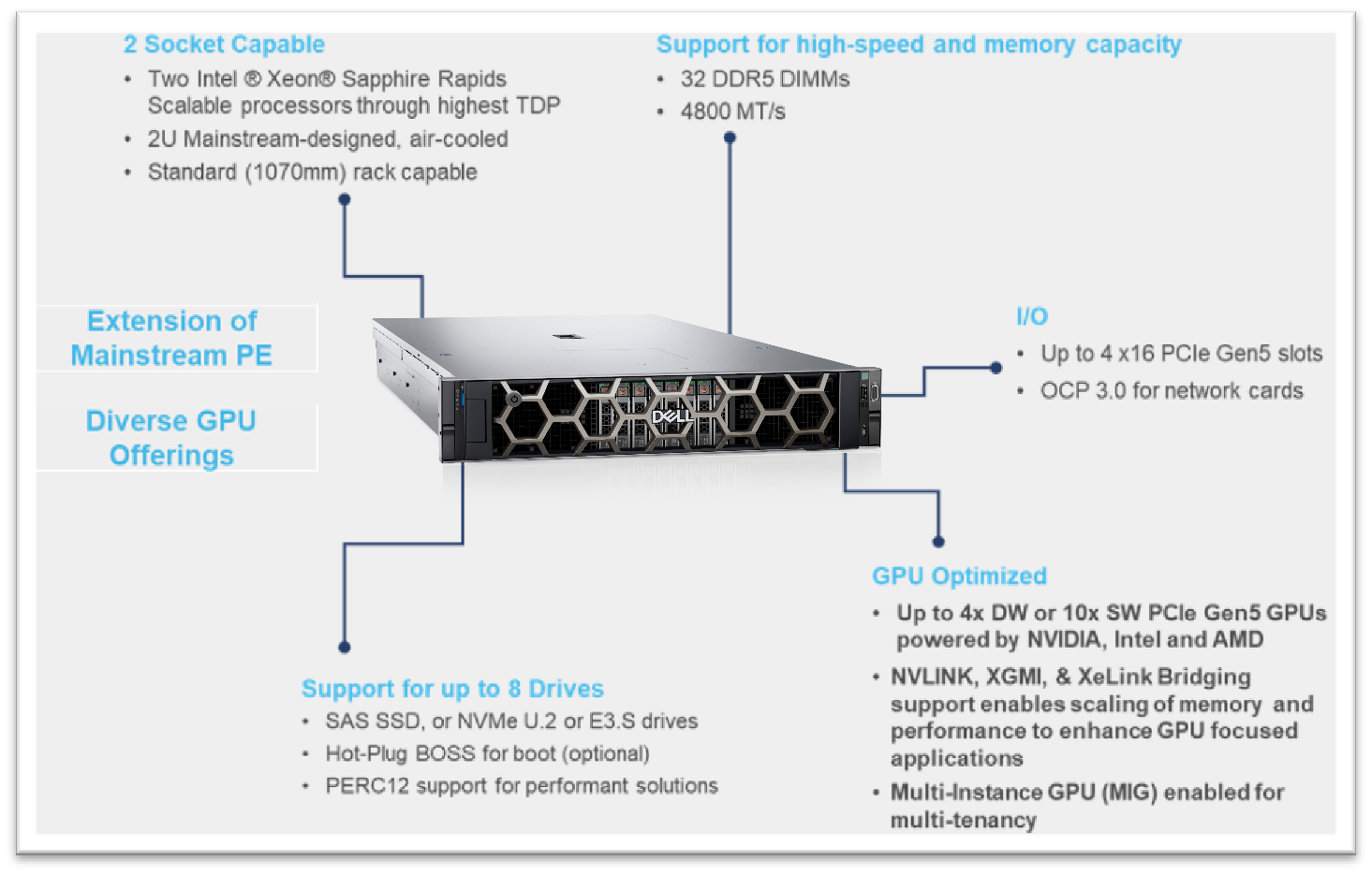
Figure 3. R760XA Specs
Table 2. Hardware and software configuration of the system
Component | Details |
Hardware | |
Compute server for inferencing | PowerEdge R760xa |
GPUs | Nvidia A100-40GB PCIe CEM GPU |
Host Processor Model Name | Intel(R) Xeon(R) Gold 6454S (Sapphire Rapids) |
Host Processors per Node | 2 |
Host Processor Core Count | 32 |
Host Processor Frequency | 2.2 GHz |
Host Memory Capacity | 512 GB, 16 x 32GB 4800 MT/s DIMMs |
Host Storage Type | SSD |
Host Storage Capacity | 900 GB |
Software | |
Operating system | Ubuntu 22.04.1 |
Profiler | |
Framework | PyTorch |
Package Management | Anaconda |
Dataset
The SAMsum dataset – size 2.94 MB – consists of approximately 16,000 rows (Train, Test, and Validation) of English dialogues and their summary. This data was used to fine-tune the Llama 2 7B model. We preprocess this data in the format of a prompt to be fed to the model for fine-tuning. In the JSON format, prompts and responses were used to train the model. During this process, PyTorch batches the data (about 10 to 11 rows per batch) and concatenates them. Thus, a total of 1,555 batches are created by preprocessing the training split of the dataset. These batches are then passed to the model in chunks for fine-tuning.
Fine-tuning steps
- Download the Llama 2 model
- The model is available either from Meta’s git repository or Hugging Face, however to access the model, you will need to submit the required registration form for Meta AI license agreement
- The details can be found in our previous work here
- Convert the model from the Meta’s git repo to a Hugging face model type in order to use the PEFT libraries used in the LoRA technique
- Use the following commands to convert the model
## Install HuggingFace Transformers from source
pip freeze | grep transformers ## verify it is version 4.31.0 or higher
git clone git@github.com:huggingface/transformers.git
cd transformers
pip install protobuf
python src/transformers/models/llama/convert_llama_weights_to_hf.py \
--input_dir /path/to/downloaded/llama/weights --model_size 7B --output_dir /output/path
- Use the following commands to convert the model
- Build a conda environment and then git clone the example fine-tuning recipes from Meta’s git repository to get started
- We have modified the code base to include Deepspeed flops profiler and nvitop to profile the GPU
- Load the dataset using the dataloader library of hugging face and, if need be, perform preprocessing
- Input the config file entries with respect to PEFT methods, model name, output directory, save model location, etc
- The following is the example code snippet
train_config: model_name: str="path_of_base_hugging_face_llama_model" run_validation: bool=True batch_size_training: int=7 num_epochs: int=1 val_batch_size: int=1 dataset = "dataset_name" peft_method: str = "lora" output_dir: str = "path_to_save_fine_tuning_model" save_model: bool = True |
6. Run the following command to perform fine tuning on a single GPU
python3 llama_finetuning.py --use_peft --peft_method lora --quantization --model_name location_of_hugging_face_model |
Figure 4 shows fine tuning with LoRA technique on 1*A100 (40GiB) with Batch size = 7 on SAMsum dataset, which took 83 mins to complete.

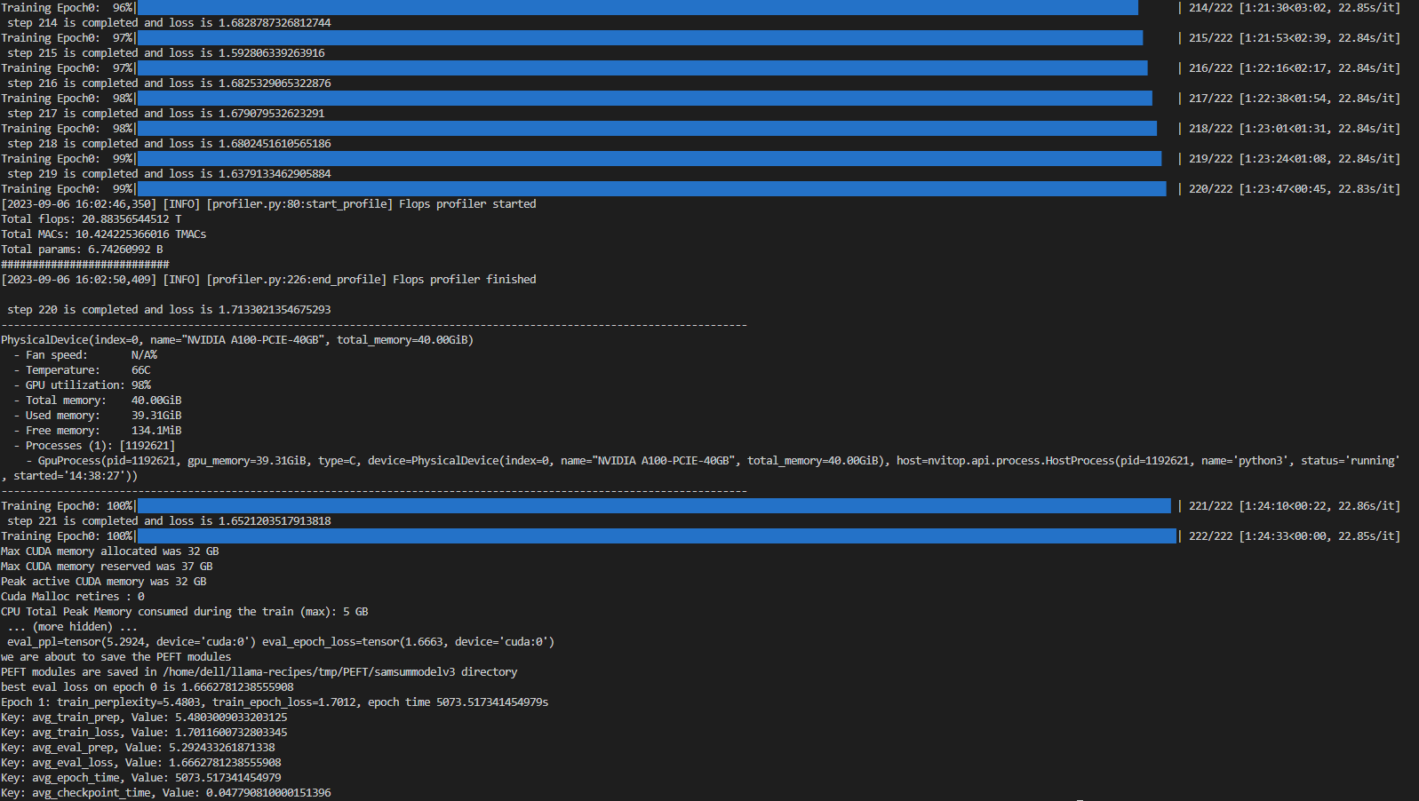
Figure 4. Example screenshot of fine-tuning with LoRA on SAMsum dataset
Experiment results
The fine-tuning experiments were run at batch sizes 4 and 7. For these two scenarios, we calculated training losses, GPU utilization, and GPU throughput. We found that at batch size 8, we encountered an out-of-memory (OOM) error for the given dataset on 1*A100 with 40 GB.
When a dialogue was sent to the base 7B model, the summarization results are not proper as shown in figure 5. After fine-tuning the base model on the SAMsum dataset, the same dialogue prompts a proper summarized result as shown in figure 6. The difference in results shows that fine-tuning succeeded.
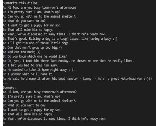
Figure 5. Summarization results from the base model.
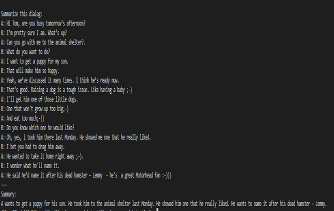
Figure 6. Summarization results from the fine-tuned model.
Figures 7 and 8 show the training losses at batch size 4 and 7 respectively. We found that even after increasing the batch size by approximately 2x times, the model training performance did not degrade.
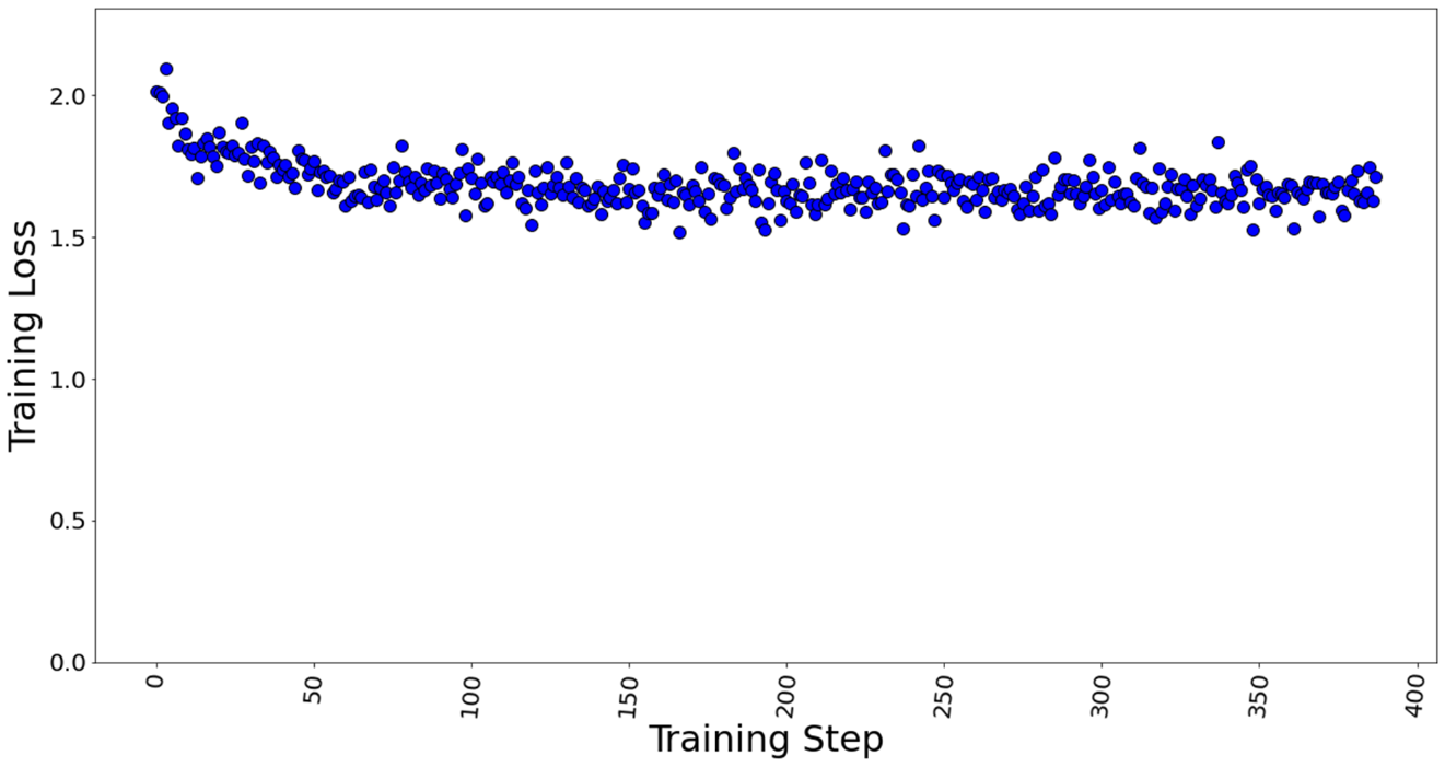
Figure 7. Training loss with batch size = 4, a total of 388 training steps in 1 epoch.
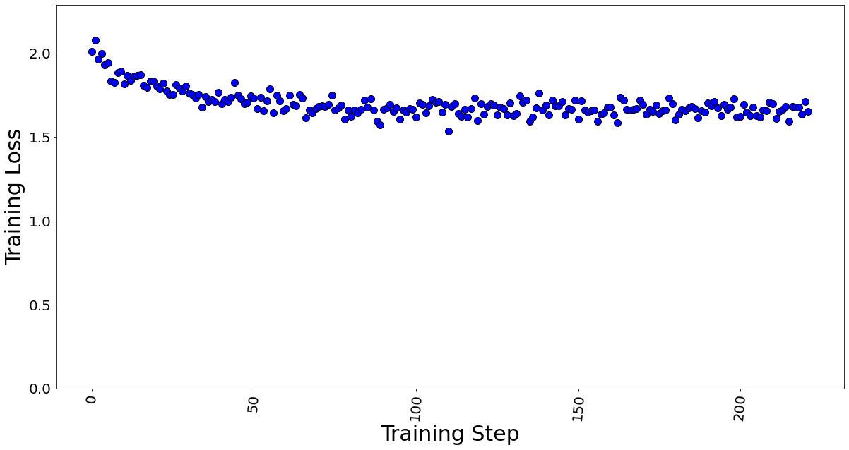
Figure 8. Training loss with batch size = 7, a total of 222 training steps in 1 epoch.
The GPU memory utilization was captured with LoRA technique in Table 3. At batch size 1, used memory was 9.31 GB. At batch size of 4, used memory was 26.21 GB. At batch size 7, memory used was 39.31 GB. Going further, we see an OOM at batch size 8 for 40 GB GPU card. The memory usage remains constant throughout fine-tuning, as shown in Figure 9, and is dependent on the batch size. We calculated the reserved memory per batch to be 4.302 GB on 1*A100.
Table 3. The GPU memory utilization is captured by varying the max. batch size parameter.
Max. Batch Size | Steps in 1 Epoch | Total Memory (GiB) | Used Memory (GiB) | Free Memory (GiB) |
1 | 1,555 | 40.00 | 9.31 | 30.69 |
4 | 388 | 40.00 | 26.21 | 13.79 |
7 | 222 | 40.00 | 39.31 | 0.69 |
8 | Out of Memory Error | |||
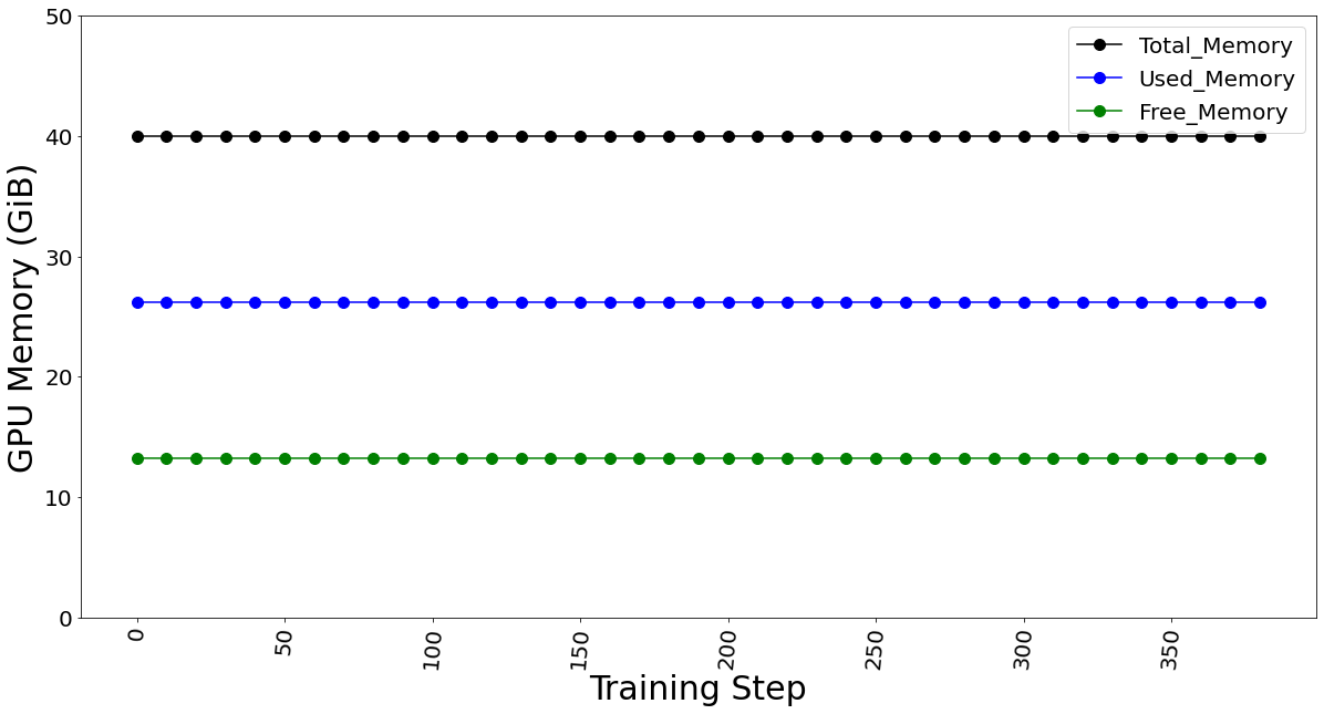
Figure 9. GPU memory utilization for batch size 4 (which remains constant for fine-tuning)
The GPU TFLOP was determined using DeepSpeed Profiler, and we found that FLOPs vary linearly with the number of batches sent in each step, indicating that FLOPs per token is the constant.
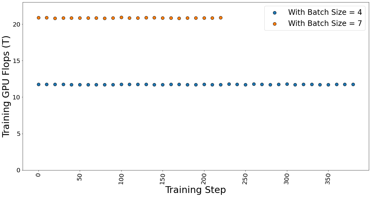
Figure 10. Training GPU TFlops for batch sizes 4 and 7 while fine-tuning the model.
The GPU multiple-accumulate operations (MACs), which are common operations performed in deep learning models, are also determined. We found that MACs also follow a linear dependency on the batch size and hence constant per token.

Figure 11. GPU MACs for batch sizes 4 and 7 while the fine-tuning the model.
The time taken for fine-tuning, which is also known as epoch time, is given in table 4. It shows that the training time does not vary much, which strengthens our argument that the FLOPs per token is constant. Hence, the total training time is independent of the batch size.
Table 4. Data showing the time taken by the fine-tuning process.
Max. Batch Size | Steps in 1 Epoch | Epoch time (secs) |
4 | 388 | 5,003 |
7 | 222 | 5,073 |
Conclusion and Recommendation
- We show that using a PEFT technique like LoRA can help reduce the memory requirement for fine-tuning a large-language model on a proprietary dataset. In our case, we use a Dell PowerEdge R760xa featuring the NVIDIA A100-40GB GPU to fine-tune a Llama 2 7B model.
- We recommend using a lower batch size to minimize automatic memory allocation, which could be utilized in the case of a larger dataset. We have shown that a lower batch size affects neither the training time nor training performance.
- The memory capacity required to fine-tune the Llama 2 7B model was reduced from 84GB to a level that easily fits on the 1*A100 40 GB card by using the LoRA technique.
Resources
- Llama 2: Inferencing on a Single GPU
- LoRA: Low-Rank Adaptation of Large Language Models
- Hugging Face Samsum Dataset
Author: Khushboo Rathi khushboo_rathi@dell.com | www.linkedin.com/in/khushboorathi
Co-author: Bhavesh Patel bhavesh_a_patel@dell.com | www.linkedin.com/in/BPat

MLPerf™ Inference 4.0 on Dell PowerEdge Server with Intel® 5th Generation Xeon® CPU


Mon, 22 Apr 2024 05:40:38 -0000
|Read Time: 0 minutes
Introduction
In this blog, we present the MLPerf™ v4.0 Data Center Inference results obtained on a Dell PowerEdge R760 with the latest 5th Generation Intel® Xeon® Scalable Processors (a CPU only system).
These new Intel® Xeon® processors use an Intel® AMX matrix multiplication engine in each core to boost overall inferencing performance. With a focus on ease of use, Dell Technologies delivers exceptional CPU performance results out of the box with an optimized BIOS profile that fully unleashes the power of Intel’s OneDNN software – a software which is fully integrated with both PyTorch and TensorFlow frameworks. The server configurations and the CPU specifications in the benchmark experiments are shown in Tables 1 and 2, respectively.
Table 1. Dell PowerEdge R760 Server Configuration
System Name | PowerEdge R760 |
Status | Available |
System Type | Data Center |
Number of Nodes | 1 |
Host Processor Model | 5th Generation Intel® Xeon® Scalable Processors |
Host Processors per Node | 2 |
Host Processor Core Count | 64 |
Host Processor Frequency | 1.9 GHz, 3.9 GHz Turbo Boost |
Host Memory Capacity | 2 TB, 16 x 128 GB 5600 MT/s |
Host Storage Capacity | 7.68TB, NVME |
Table 2. 5th Generation Intel® Xeon® Scalable Processor Technical Specifications
Product Collection | 5th Generation Intel® Xeon® Scalable Processors |
Processor Name | Platinum 8592+ |
Status | Launched |
# of CPU Cores | 64 |
# of Threads | 128 |
Base Frequency | 1.9 GHz |
Max Turbo Speed | 3.9 GHz |
Cache L3 | 320 MB |
Memory Type | DDR5 5600 MT/s |
ECC Memory Supported | Yes |
MLPerf™ Inference v4.0 - Datacenter
The MLPerf™ inference benchmark measures how fast a system can perform ML inference using a trained model with new data in a variety of deployment scenarios. There are two benchmark suites, one for Datacenter systems and one for Edge. Figure 1 shows the 7 models with each targeting at different task in the official release v4.0 for Datacenter systems category that were run on this PowerEdge R760 and submitted in the closed category. The dataset and quality target are defined for each model for benchmarking, as listed in Table 3.
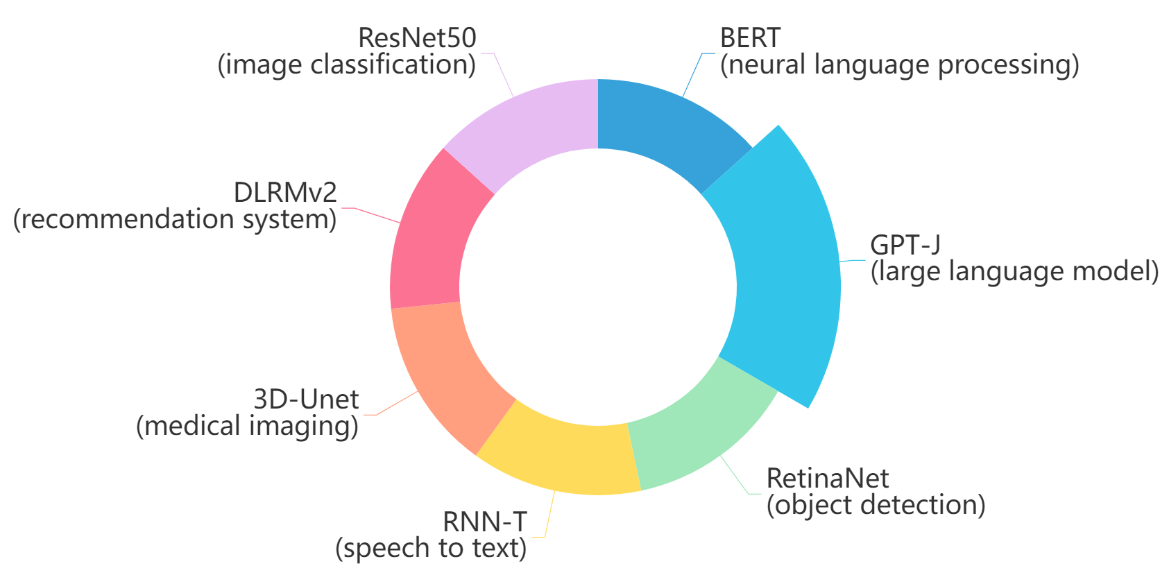
Figure 1. Benchmarked models for MLPerf™ datacenter inference v4.0
Table 3. Datacenter Suite Benchmarks. Source: MLCommons™
Area | Task | Model | Dataset | QSL Size | Quality | Server latency constraint |
Vision | Image classification | ResNet50-v1.5 | ImageNet (224x224) | 1024 | 99% of FP32 (76.46%) | 15 ms |
Vision | Object detection | RetinaNet | OpenImages (800x800) | 64 | 99% of FP32 (0.20 mAP) | 100 ms |
Vision | Medical imaging | 3D-Unet | KITS 2019 (602x512x512) | 16 | 99.9% of FP32 (0.86330 mean DICE score) | N/A |
Speech | Speech-to-text | RNN-T | Librispeech dev-clean (samples < 15 seconds) | 2513 | 99% of FP32 (1 - WER, where WER=7.452253714852645%) | 1000 ms |
Language | Language processing | BERT-large | SQuAD v1.1 (max_seq_len=384) | 10833 | 99% of FP32 and 99.9% of FP32 (f1_score=90.874%) | 130 ms |
Language | Summarization | GPT-J | CNN Dailymail (v3.0.0, max_seq_len=2048) | 13368 | 99% of FP32 (f1_score=80.25% rouge1=42.9865, rouge2=20.1235, rougeL=29.9881). | 20 s |
Commerce | Recommendation | DLRMv2 | Criteo 4TB multi-hot | 204800 | 99% of FP32 (AUC=80.25%) | 60 ms |
Scenarios
The models are deployed in a variety of critical inference applications or use cases known as “scenarios” where each scenario requires different metrics, demonstrating production environment performance in practice. Following is the description of each scenario. Table 4 shows the scenarios required for each Datacenter benchmark included in this submission v4.0.
Offline scenario: represents applications that process the input in batches of data available immediately and do not have latency constraints for the metric performance measured in samples per second.
Server scenario: represents deployment of online applications with random input queries. The metric performance is measured in queries per second (QPS) subject to latency bound. The server scenario is more complicated in terms of latency constraints and input queries generation. This complexity is reflected in the throughput-degradation results compared to the offline scenario.
Each Datacenter benchmark requires the following scenarios:
Table 4. Datacenter Suite Benchmark Scenarios. Source: MLCommons™
Area | Task | Required Scenarios |
Vision | Image classification | Server, Offline |
Vision | Object detection | Server, Offline |
Vision | Medical imaging | Offline |
Speech | Speech-to-text | Server, Offline |
Language | Language processing | Server, Offline |
Language | Summarization | Server, Offline |
Commerce | Recommendation | Server, Offline |
Software stack and system configuration
The software stack and system configuration used for this submission is summarized in Table 5.
Table 5. System Configuration
OS | CentOS Stream 8 (GNU/Linux x86_64) |
Kernel | 6.7.4-1.el8.elrepo.x86_64 |
Intel® Optimized Inference SW for MLPerf™ | MLPerf™ Intel® OneDNN integrated with Intel® Extension for PyTorch (IPEX) |
ECC memory mode | ON |
Host memory configuration | 2TB, 16 x 128 GB, 1 DIMM per channel, well balanced |
Turbo mode | ON |
CPU frequency governor | Performance |
What is Intel® AMX (Advanced Matrix Extensions)?
Intel® AMX is a built-in accelerator that enables 5th Gen Intel® Xeon® Scalable processors to optimize deep learning (DL) training and inferencing workloads. With the high-speed matrix multiplications enabled by Intel® AMX, 5th Gen Intel® Xeon® Scalable processors can quickly pivot between optimizing general computing and AI workloads.
Imagine an automobile that could excel at city driving and then quickly shift to deliver Formula 1 racing performance. 5th Gen Intel® Xeon® Scalable processors deliver this level of flexibility. Developers can code AI functionality to take advantage of the Intel® AMX instruction set as well as code non-AI functionality to use the processor instruction set architecture (ISA). Intel® has integrated the oneAPI Deep Neural Network Library (oneDNN) – its oneAPI DL engine – into popular open-source tools for AI applications, including TensorFlow, PyTorch, PaddlePaddle, and ONNX.
AMX architecture
Intel® AMX architecture consists of two components, as shown in Figure 1:
- Tiles consist of eight two-dimensional registers, each 1 kilobyte in size. They store large chunks of data.
- Tile Matrix Multiplication (TMUL) is an accelerator engine attached to the tiles that performs matrix-multiply computations for AI.
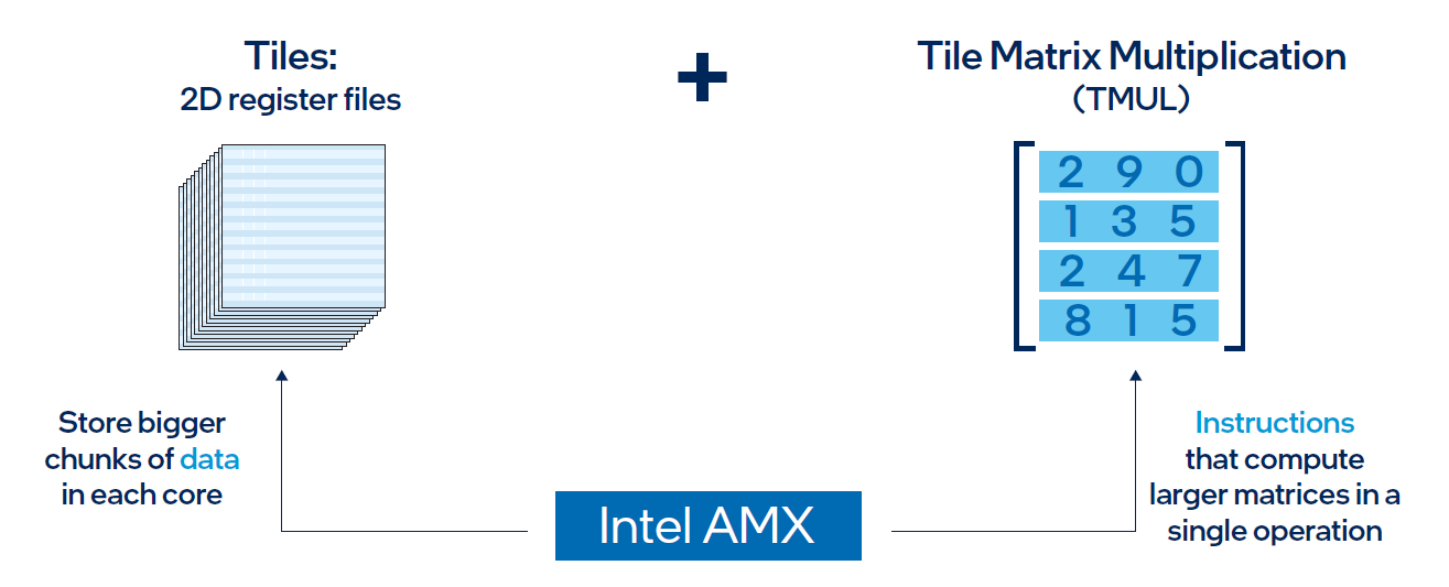
Figure 2. Intel® AMX architecture consists of 2D register files (tiles) and TMUL
Results
Both MLPerf™ v3.1 and MLPerf™ v4.0 benchmark results are based on the Dell R760 server but with different generations of Xeon® CPUs (4th Generation Intel® Xeon® CPUs for MLPerf™ v3.1 versus 5th Generation Intel® Xeon® CPUs for MLPerf™ v4.0) and optimized software stacks. In this section, we show the performance in the comparing mode so the improvement from the last submission can be easily observed.
Comparing Performance from MLPerfTM v4.0 to MLPerfTM v3.1
ResNet50 server & offline scenarios:
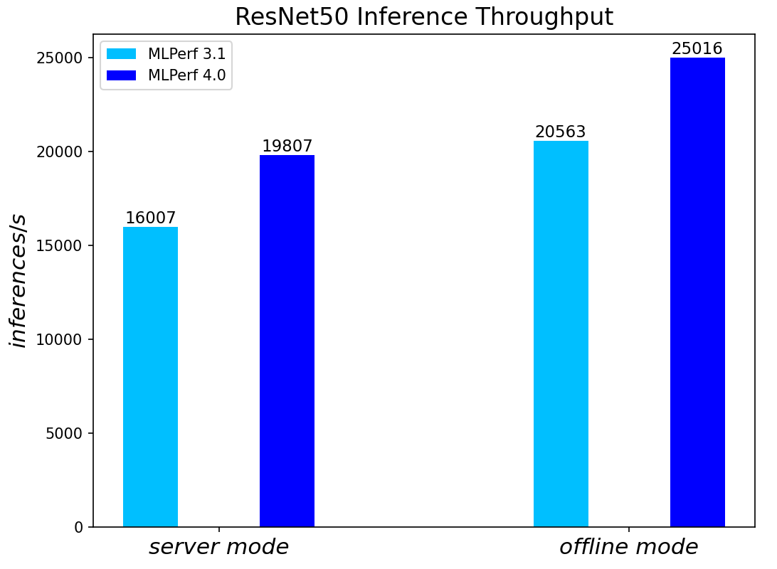
Figure 3. ResNet50 inference throughput in server and offline scenarios
BERT Large Language Model server & offline scenarios:
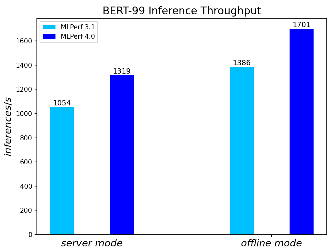
Figure 4. BERT Inference results for server and offline scenarios
RetinaNet Object Detection Model server & offline scenarios:
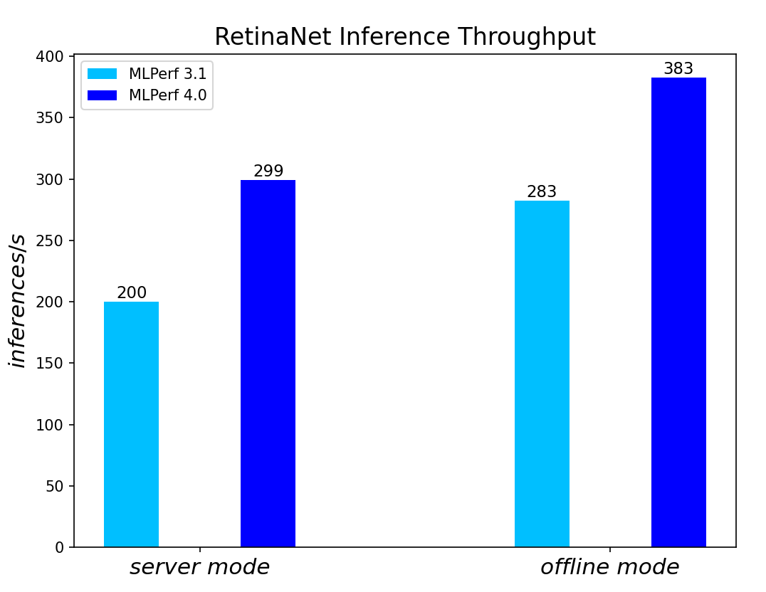
Figure 5. RetinaNet Object Detection Model Inference results for server and offline scenarios
RNN-T Text to Speech Model server & offline scenarios:
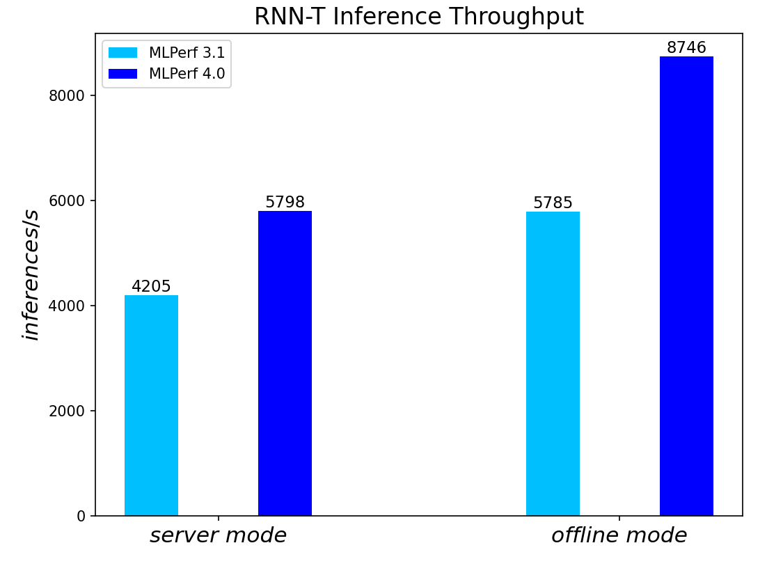
Figure 6. RNN-T Text to Speech Model Inference results for server and offline scenarios
3D-Unet Medical Imaging Model offline scenarios:
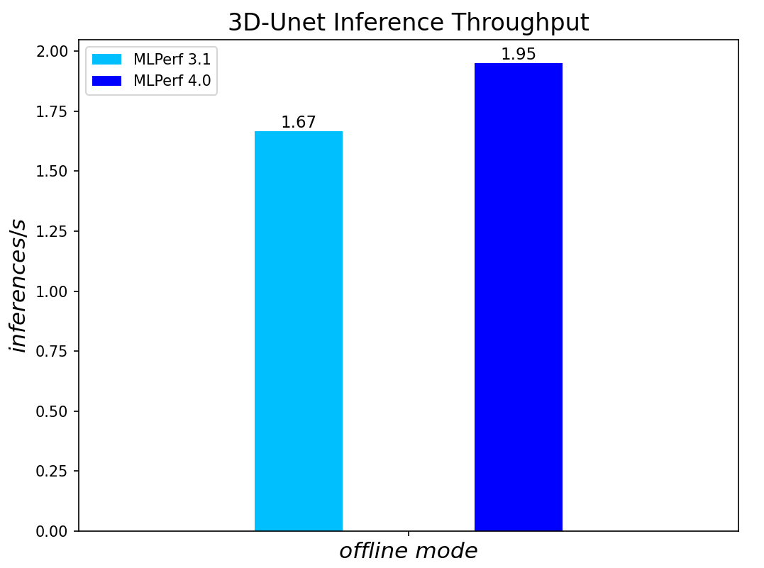
Figure 7. 3D-Unet Medical Imaging Model Inferencing results for server and offline scenarios
DLRMv2-99 Recommendation Model server & offline scenarios:
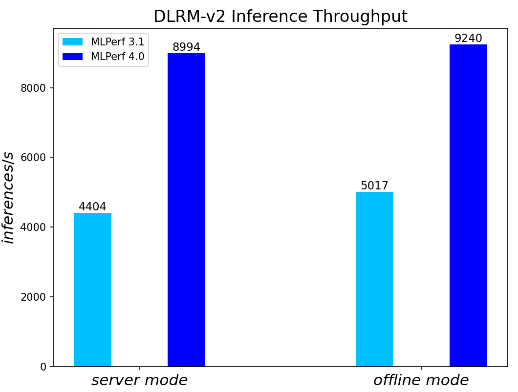
Figure 8. DLRMv2-99 Recommendation Model Inference results for server and offline scenarios
GPT-J-99 Summarization Model server & offline scenarios:
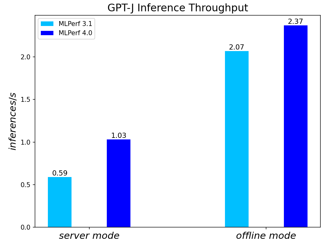
Figure 9. GPT-J-99 Summarization Model Inference results for server and offline scenarios
Conclusion
- The PowerEdge R760 server with 5th Generation Intel® Xeon® Scalable Processors produces strong data center inference performance, confirmed by the official version 4.0 MLPerfTM benchmarking results from MLCommonsTM.
- The high performance and versatility are demonstrated across natural language processing, image classification, object detection, medical imaging, speech-to-text inference, recommendation, and summarization systems.
- Compared to its prior version 3.0 and 3.1 submissions enabled by 4th Generation Intel® Xeon® Scalable Processors, the R760 with 5th Generation Intel® Xeon® Scalable Processors show significant performance improvement across different models, including the generative AI models like GPT-J.
- The R760 supports different deep learning inference scenarios in the MLPerfTM benchmark scenarios as well as other complex workloads such as database and advanced analytics. It is an ideal solution for data center modernization to drive operational efficiency, lead to higher productivity, and minimize total cost of ownership (TCO).
References
MLCommonsTM MLPerfTM v4.0 Inference Benchmark Submission IDs
ID | Submitter | System |
4.0-0026 | Dell | Dell PowerEdge Server R760 (2x Intel® Xeon® Platinum 8592+) |

Dell and Northwestern Medicine Collaborate on Next Generation Healthcare Multimodal LLMs
Thu, 15 Feb 2024 15:56:13 -0000
|Read Time: 0 minutes
Generative multimodal large language models, or mLLMs, have shown remarkable new capabilities across a variety of domains, ranging from still images to video to waveforms to language and more. However, the impact of healthcare-targeted mLLM applications remains untried, due in large part to the increased risks and heightened regulation encountered in the patient care setting. A collaboration between Dell Technologies and Northwestern Medicine aims to pave the way for the development and integration of next-generation healthcare-oriented mLLMs into hospital workflows via a strategic partnership anchored in technical and practical expertise at the intersection of healthcare and technology.
One practical application of mLLMs is highlighted in a recent open-source publication from the Research and Development team at Northwestern Medicine which describes the development and evaluation of an mLLM for the interpretation of chest x-rays. These interpretations were judged by emergency physicians to be as accurate and relevant in the emergency setting as interpretations by on-site radiologists, even surpassing teleradiologist interpretations. Clinical implementation of such a model could broaden access to care while aiding physician decision-making. This peer-reviewed study – the first to clinically evaluate a generative mLLM for chest x-ray interpretation – is just one example of the numerous opportunities for meaningful impact by healthcare-tailored mLLMs.
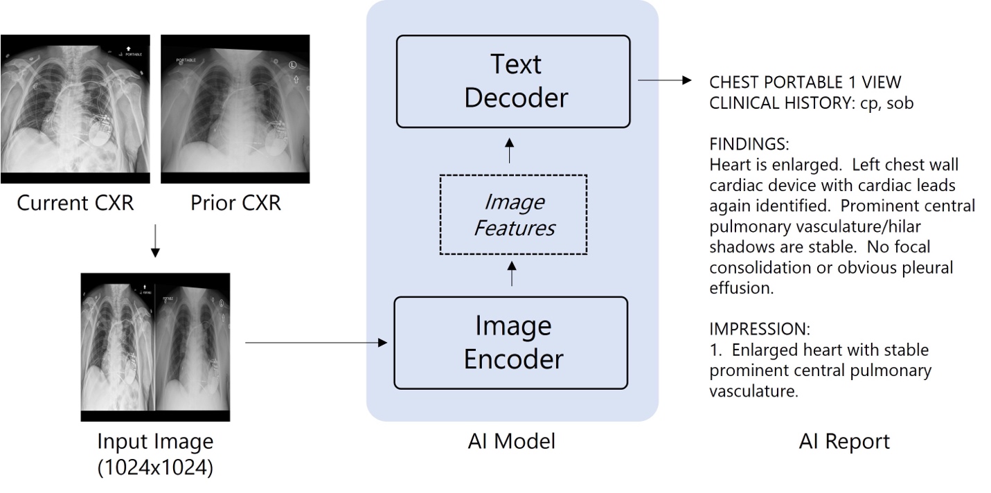 Figure 1. Model architecture for chest x-ray interpretation
As illustrated in Figure 1, the model is a vision encoder-decoder model, using pretrained ViT-base and RoBERTa-base as the image encoder and text decoder respectively. In total, over 1 million images and radiology reports were used to train this model using one node with 8 GPUs over three weeks. Expanding the scope of such models, such as to other image modalities like computed tomography and magnetic resonance imaging, requires much greater hardware capabilities to efficiently train at scale.
Notably, this model was trained using only 8 graphics processing units (GPUs) in three weeks. As the broader body of LLM research has shown, there is great promise in scaling up such methods, incorporating more data and larger models to create more powerful solutions. Hospital systems generate vast amounts of data spanning numerous modalities, such as numeric lab values, clinical images and videos, waveforms, and free text clinical notes. A key goal of the collaboration between Dell Technologies and Northwestern Medicine is to expand on this work and scale the capabilities of healthcare systems to use their own data to solve clinical problems and blend cutting edge data-centric platforms with clinical expertise, all targeted toward improving the patient and practitioner experience.
HIPAA Compliant HPC
To bring this vision to fruition, it is necessary to build out capable healthcare-tailored high-performance computing (HPC) clusters in which multiple nodes with varying levels of compute, memory, and storage resources are made available to users to run tasks in parallel and at scale. This enables centralized management of resources with the flexibility to provision resources to jobs ranging from single-node experiments to massively distributed model training. The typical HPC cluster structure is illustrated in Figure 2. Users can connect to a login node via virtual private network (VPN) or secure shell (SSH). These nodes provide access to requested compute resources within the internal HPC cluster network as well as job scheduling software, such as slurm, to coordinate job submission and distribution. Computing nodes are interconnected with varying levels of provisioned access available, ranging from one GPU on a multi-GPU node to dozens of multi-GPU nodes. A shared parallel filesystem is used to access the data storage.
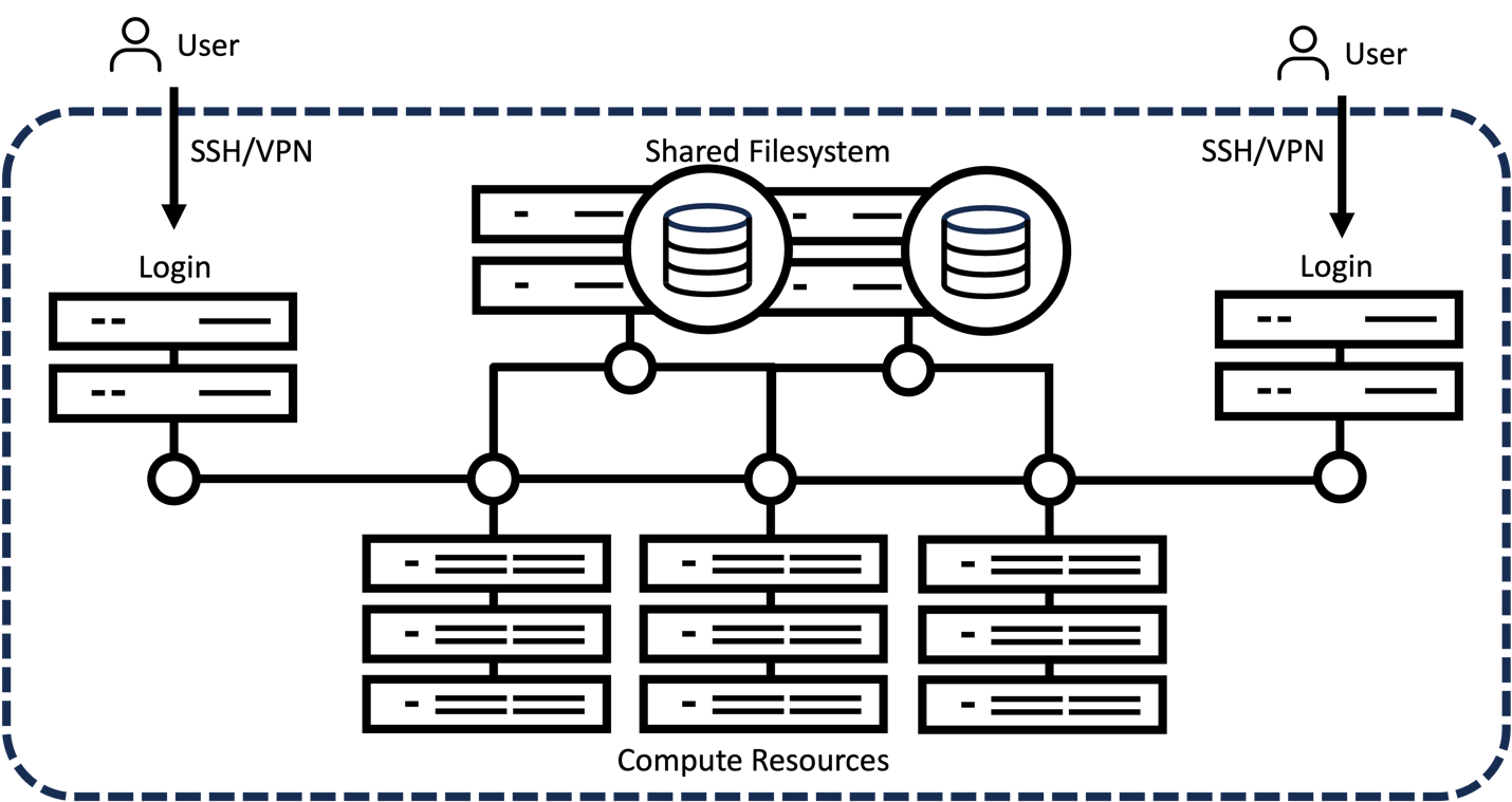 Figure 2. Typical HPC cluster setup
However, a special consideration within ecosystems handling hospital data is protected health information, or PHI. The Health Insurance Portability and Accountability Act, or HIPAA, mandates a basic level of security to ensure that PHI is adequately protected, ensuring patient privacy around sensitive health data. Thus, HIPAA-compliant healthcare HPC must account for heightened security and segregation of PHI. But what exactly does it mean to be HIPAA compliant? The following will describe some key components necessary to ensure HIPAA compliance and protection of sensitive patient data throughout all aspects of hospital-based collaborations. Though HIPAA compliance may seem challenging, we break down these requirements into two key facets: the data silo and data stewardship, as shown in Figure 3.
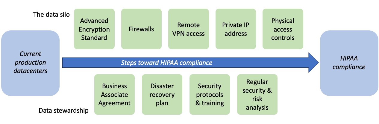 Figure 3. The key facets needed to ensure HIPAA compliance in datacenters housing healthcare data
Firstly, the data silo must ensure that access is provisioned in a secure and controllable fashion. Data must be encrypted in accordance with the Advanced Encryption Standard (AES), such as by AES-256 which utilizes a 256-bit key. Adequate firewalls, a private IP address, and access via remote VPN are further required to ensure that PHI remains accessible only to authorized parties and in a secure fashion. Finally, physical access controls ensure credentialed access and surveillance within the datacenter itself.
Secondly, data stewardship practices must be in place to ensure that practices remain up to date and aligned with institutional goals. A business associate agreement (BAA) describes the responsibilities of each party with regards to protection of PHI in a legally binding fashion and is necessary if business associate operations require PHI access. Security protocols, along with a disaster recovery plan, should be outlined to ensure protection of PHI in all scenarios. Finally, regular security and risk analyses should be performed to maintain compliance with applicable standards and identify areas of improvement.
While many datacenters have implemented measures to ensure compliance with regulations like HIPAA, the greatest challenge remains providing on-demand separation between general workloads and HIPAA-compliant workloads within the same infrastructure. To address this issue, Dell Technologies is working in collaboration with Northwestern Medicine on a new approach that utilizes flexible, controlled provisioning to enable on-demand HIPAA compliance within existing HPC clusters, as shown in Figure 4. This HPC setup, once deployed, would automatically provide network separation and the reconfiguration of compute and data storage resources, ensuring they are isolated from the general allocation.
This newly HIPAA-compliant portion of the cluster can be accessed only by credentialed users via VPN using dedicated login nodes which provide separate job scheduling and filesystem access, enabling access to AI-ready compute resources without disrupting general workloads. When no longer needed, automatic cluster reconfiguration occurs, returning resources to the general allocation until new HIPAA-compliant workloads are needed.
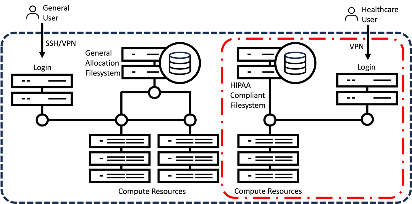 Figure 4. Next-generation HIPAA-compliant HPC cluster, which builds on the typical setup presented in Figure 1
Our expertise in compute infrastructure for artificial intelligence (AI) initiatives extends to developing datacenters and datacenter infrastructure with the proper security and controls in place that a health system can leverage as part of their efforts in achieving HIPAA compliance.
This integrated model of HIPAA-compliant compute for healthcare is aimed at democratizing the benefits of the artificial intelligence revolution, enabling healthcare institutions to employ these new technologies and provide better, more efficient care for all.
Resources
Generative Artificial Intelligence for Chest Radiograph Interpretation in the Emergency Department: https://jamanetwork.com/journals/jamanetworkopen/fullarticle/2810195
Author:
Jonathan Huang, MD/PhD Candidate, Research & Development, Northwestern Medicine
Matthew Wittbrodt, Solutions Architect, Research & Development, Northwestern Medicine
Alex Heller, Director, Research & Development, Northwestern Medicine
Mozziyar Etemadi, Clinical Director, Advanced Technologies, Northwestern Medicine
Bhavesh Patel, Sr. Distinguished Engineer, Dell Technologies
Bala Chandrasekaran, Technical Staff, Dell Technologies
Frank Han, Senior Principal Engineer, Dell Technologies
Steven Barrow, Enterprise Account Executive

Investigating the Memory Access Bottlenecks of Running LLMs
Thu, 18 Jan 2024 20:20:03 -0000
|Read Time: 0 minutes
Introduction
Memory access and computing are the two main functions in any computer system. In past decades, the computing capability of a processor has greatly benefited from Moore’s Law which brings smaller and faster transistors into the silicon die almost every year. On the other hand, system memory is regressing. The trend of shrinking fabrication technology for a system is making memory access much slower. This imbalance causes the computer system performance to be bottle-necked by the memory access; this is referred to as the “memory wall” issue. The issue gets worse for large language model (LLM) applications, because they require more memory and computing. Therefore, more memory access is required to be able to execute those larger models.
In this blog, we will investigate the impacts of memory access bottlenecks to the LLM inference results. For the experiments, we chose the Llama2 chat models running on a Dell PowerEdge HS5610 server with the 4th Generation Intel® Xeon® Scalable Processors. For quantitative analysis, we will be using the Intel profile tool – Intel® VTune™ Profiler to capture the memory access information while running the workload. After identifying the location of the memory access bottlenecks, we propose the possible techniques and configurations to mitigate the issues in the conclusion session.
Background
The Natural Language Processing (NLP) has greatly benefited from the transformer architecture since it was introduced in 2017 [1]. The trajectory of the NLP models has been moved to transformer-based architectures given its parallelization and scalability features over the traditional Recurrent Neural Networks (RNN) architectures. Research shows a scaling law of the transformer-based language models, in which the accuracy is strongly related to the model size, dataset size and the amount of compute [2]. This inspired the interest in using Large Language Models (LLMs) for high accuracy and complicated tasks. Figure 1 shows the evolution of the LLMs since the transformer architecture was invented. We can see the parameters of the LLMs have increased dramatically in the last 5 years. This trend is continuing. As shown in the figure, most of the LLMs today come with more than 7 billion parameters. Some models like GPT4 and PaLM2 have trillion-level parameters to support multi-mode features.
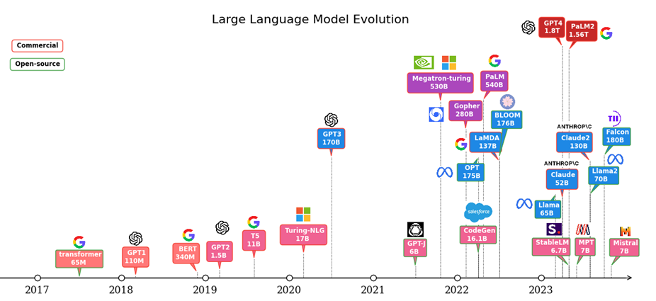
Figure 1: LLM evolution
What comes with the large models are the challenges on the hardware systems for training and inferencing those models. On the one hand, the computation required is tremendous as it is proportional to the model size. On the other hand, memory access is expensive. This mainly comes from the off-chip communication and complicated cache architectures required to support the large model parameters and computation.
Test Setup
The hardware platform we used for this study is HS5610 which is the latest 16G cloud-optimized server from Dell product portfolio. Figure 2 gives an overview of HS5610. It has been designed with CSP features that allow the same benefits with full PowerEdge features & management like mainstream Dell servers, as well as open management (OpenBMC), cold aisle service, channel firmware, and services. The server has two sockets with an Intel 4th generation 32-core Intel® Xeon® CPU on each socket. The TDP power for each CPU is 250W. Table 1 and Table 2 show the details of the server configurations and CPU specifications.
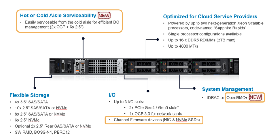
Figure 2: PowerEdge HS5610 [3]
Product Collection | 4th Generation Intel® Xeon® Scalable Processors |
Processor Name | Platinum 8480+ |
Status | Launched |
# of CPU Cores | 32 |
# of Threads | 64 |
Base Frequency | 2.0 GHz |
Max Turbo Speed | 3.8 GHz |
Cache L3 | 64 MB |
Memory Type | DDR5 4800 MT/s |
ECC Memory Supported | Yes |
Table 1: HS5610 Server Configurations
System Name | PowerEdge HS5610 |
Status | Available |
System Type | Data Center |
Number of Nodes | 1 |
Host Processor Model | 4th Generation Intel® Xeon® Scalable Processors |
Host Processors per Node | 2 |
Host Processor Core Count | 32 |
Host Processor Frequency | 2.0 GHz, 3.8 GHz Turbo Boost |
Host Memory Capacity | 1TB, 16 x 64GB DIMM 4800 MHz |
Host Storage Capacity | 4.8 TB, NVME |
Table 2: 4th Generation 32-core Intel® Xeon® Scalable Processor Technical Specifications
Software Stack and System Configuration
The software stack and system configuration used for this submission is summarized in Table 3. Optimizations have been done for the PyTorch framework and Transformers library to unleash the Xeon CPU AI instruction capabilities. Also, a low-level tool - Intel® Neural Compressor has been used for high-accuracy quantization.
OS | CentOS Stream 8 (GNU/Linux x86_64) |
Intel® Optimized Inference SW | OneDNN™ Deep Learning, ONNX, Intel® Extension for PyTorch (IPEX), Intel® Extension for Transformers (ITREX), Intel® Neural Compressor |
ECC memory mode | ON |
Host memory configuration | 1TiB |
Turbo mode | ON |
CPU frequency governor | Performance |
Table 3: Software stack and system configuration
The model under tests is Llama2-chat-hf models with 13 billion parameters (Llama2-13b-chat-hf). The model is based on the pre-trained 13 billion Llama2 model and fine-tuned with human feedback for chatbot applications. The Llama2 model has light (7b), medium (13b) and heavy (70b) size versions.
The profile tool used in the experiments is Intel® VTune™. It is a powerful low-level performance analysis tool for x86 CPUs that supports algorithms, micro-architecture, parallelism, and IO related analysis etc. For the experiments, we use the memory access analysis under micro-architecture category. Note Intel® VTune™ consumes significant hardware resources which impacts the performance results if we run the tool along with the workload. So, we use it as a profile/debug tool to investigate the bottleneck. The performance numbers we demonstrate here are running without Intel® VTune™ on.
The experiments are targeted to cover the following:
- Single-socket performance vs dual-socket performance to demonstrate the NUMA memory access impact.
- Performance under different CPU-core numbers within a single socket to demonstrate the local memory access impact.
- Performance with different quantization to demonstrate the quantization impact.
- Intel® VTune™ memory access results.
Because Intel® VTune™ has minimum capture durations and max capture size requirements, we focus on capturing the results for the medium-size model (Llama2-13b-chat-hf). This prevents short/long inference time therefore avoiding an underload or overload issue. All the experiments are based on the batch size equals to 1. Performance is characterized by latency or throughput. To reduce the measurement errors, the inference is executed 10 times to get the averaged value. A warm-up process by loading the parameter and running a sample test is executed before running the defined inference.
Results
For this section, we showcase the performance results in terms of throughput for single-socket and dual socket scenarios under different quantization types followed by the Intel® VTune™ capturing results.
Single-socket Results Under Different Quantization Types:
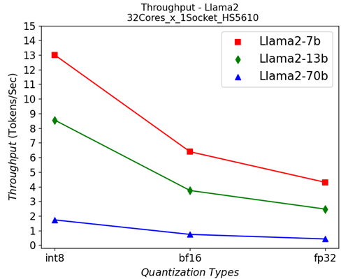
Figure 3: Single-socket throughput in HS5610 server running Llama2 models under different quantization types
Figure 3 shows the throughputs of running different Llama2 chat models with different quantization types on a single socket. The “numactl” command is used to confine the workload within one single 32-core CPU. From the results, we can see that quantization greatly helps to improve the performance across different models.
 |  |
(a) | (b) |
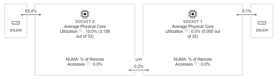
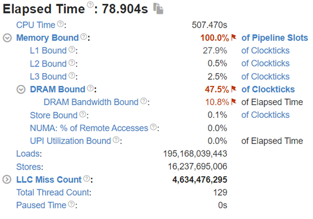
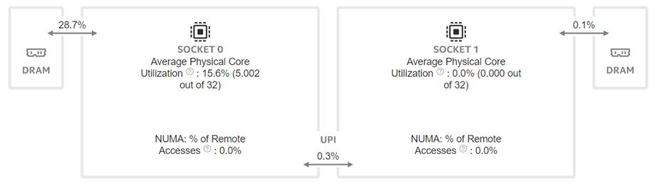
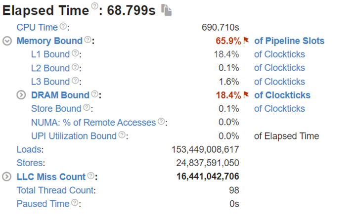
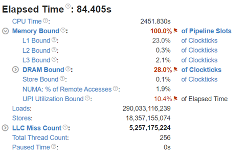
Figure 4:Intel® VTune™ memory analysis results for single-socket fp32 results:
(a). bandwidth and utilization diagram (b). elapsed time analysis
 |  |
(a) | (b) |
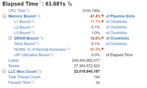
Figure 5: Intel® VTune™ memory analysis results for single-socket bf16 results:
(a). bandwidth and utilization diagram (b). elapsed time analysis
To better understand what would happen at the lower level, we will take the Llama2 13 billion model as an example. We will use Intel® VTune™ to capture the bandwidth and utilization diagram and the elapsed time analysis for the fp32 data type (shown in Figure 4) and use bf16 data type (shown in Figure 5). We can see that by reducing the representing bits, the bandwidth required for the CPU and DRAM communication is reduced. In this scenario, the DRAM utilization drops from 63.4% for fp32 (shown in Figure 4 (a)) to 28.7% (shown in Figure 4 (b)). The also indicates that the weight data can arrive quicker to the CPU chip. Now we can benefit from the quicker memory communication. The CPU utilization also increases from 10% for fp32 (shown in Figure 4 (a)) to 15.6% for bf16 (shown in Figure 4 (b)). Both faster memory access and better CPU utilization translate to better performance with a more than 50% (from 2.47 tokens/s for fp32 to 3.74 tokens/s) throughput boost as shown in Figure 3. Diving deeper with the elapsed time analysis shown in Figure 4 (b), and Figure 5 (b), L1 cache is one of the performance bottleneck locations on the chip. Quantization reduces the possibility that the task gets stalled.
Dual-socket Results Under Different Quantization Types:
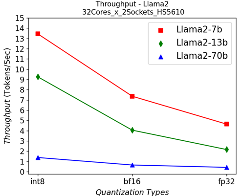
Figure 6: Dual-socket throughput in HS5610 server running Llama2 models under different quantization types
 |  |
(a) | (b) |
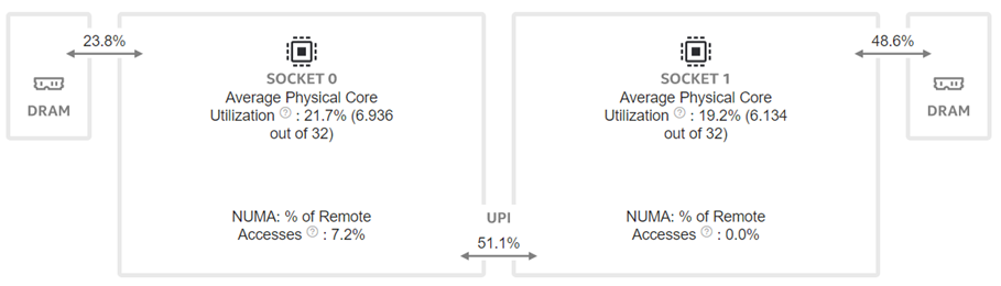
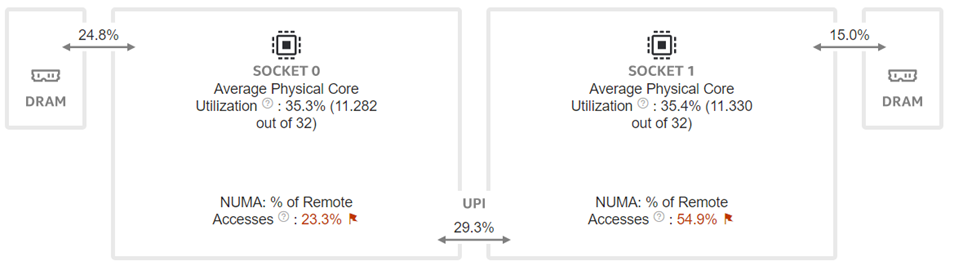
Figure 7: Intel® VTune™ memory analysis results for dual-socket fp32 results:
(a). bandwidth and utilization diagram (b). elapsed time analysis
 |  |
(a) | (b) |
Figure 8: Intel® VTune™ memory analysis results for dual-socket bf16 results:
(a). bandwidth and utilization diagram (b). elapsed time analysis
Now moving to the dual-socket scenarios shown in Figure 6-8, we have similar observations regarding the impacts of the quantization: Quantization increases CPU utilization and reduces the L1 cache bottleneck, therefore boosting the throughputs across different Llama2 models.
Comparing the performance between the single-socket (shown in Figure 3) and dual-socket (shown in Figure 6) scenarios indicates negligible performance improvement. As seen in Figure 7 and 8, even though we get better CPU utilizations, the communication between two sockets (the UPI or the NUMA memory access), becomes the main bottleneck that offsets the benefits of having more computing cores.
Conclusion
Based on the experiment results for different Llama2 models under various configurations, we have the conclusions as the following:
- Quantization improves the performance across the models with different weights by reducing the L1 cache bottleneck and increasing the CPU utilization. It also indicates that we can optimize the TCO by reducing the memory requirements (in terms of the capacity and speed) if we were able to quantize the model properly.
- Crossing-socket communication from either UPI or NUMA memory access is a significant bottleneck that may affect performance. Optimizations include the reducing of the inter-socket communication. For example better partitioning of the model is critical. Alternatively, this also indicates that executing one workload on a single dedicated CPU with enough cores is desirable for cost and performance considerations.
References
[1]. A. Vaswani et. al, “Attention Is All You Need”, https://arxiv.org/abs/1706.03762
[2]. J. Kaplan et. al, “Scaling Laws for Neural Language Models”, https://arxiv.org/abs/2001.08361
[3]. https://www.dell.com/en-us/shop/ipovw/poweredge-hs5610

Deploying Llama 7B Model with Advanced Quantization Techniques on Dell Server
Tue, 16 Jan 2024 20:05:01 -0000
|Read Time: 0 minutes
Introduction
Large-language Models (LLMs) have gained great industrial and academic interest in recent years. Different LLMs have been adopted in various applications, such as: content generation, text summarization, sentiment analysis, and healthcare. The LLM evolution diagram in Figure 1 shows the popular pre-trained models since 2017 when the transformer architecture was first introduced [1]. It is not hard to find the trend of larger and more open-source models following the timeline. Open-source models boosted the popularity of LLMs by eliminating the huge training cost associated with the large scale of the infrastructure and long training time required. Another portion of the cost of LLM applications comes from the deployment where an efficient inference platform is required.
This blog focuses on how to deploy LLMs efficiently on Dell platform with different quantization techniques. We first benchmarked the model accuracy under different quantization techniques. Then we demonstrated their performance and memory requirements of running LLMs under different quantization techniques through experiments. Specifically, we chose the open-source model Llama-2-7b-chat-hf for its popularity [2]. The server is chosen to be Dell main-stream server R760xa with NVIDIA L40 GPUs [3] [4]. The deployment framework in the experiments is TensorRT-LLM, which enables different quantization techniques including advanced 4bit quantization as demonstrated in the blog [5].
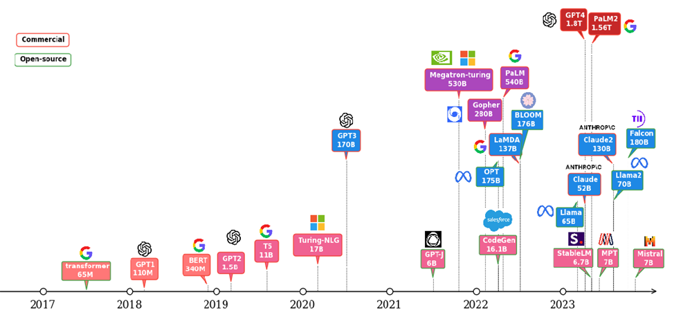
Figure 1 :LLM evolution
Background
LLM inferencing processes tend to be slow and power hungry, because of the characteristics of LLMs being large in weight size and having auto-regression. How to make the inferencing process more efficient under limited hardware resources is among the most critical problems for LLM deployment. Quantization is an important technique widely used to push for more efficient LLM deployment. It can relieve the large hardware resource requirements by reducing the memory footprint and computation energy, as well as improve the performance with faster memory access time compared to the deployment with the original un-quantized model. For example, in [6], the performance in terms of throughput by tokens per second (tokens/s) for Llama-2-7b model is improved by more than 2x by quantizing from floating point 16-bit format to integer 8-bit. Recent research made more aggressive quantization techniques like 4-bit possible and available in some deployment frameworks like TensorRT-LLM. However, quantization is not free, and it normally comes with accuracy loss. Besides the cost, reliable performance with acceptable accuracy for specific applications is what users would care about. Two key topics covered in this blog are accuracy and performance. We first benchmark the accuracy of the original model and quantized models over different tasks. Then we deployed those models into Dell server and measured their performance. We further measured the GPU memory usage for each scenario.
Test Setup
The model under investigation is Llama-2-7b-chat-hf [2]. This is a finetuned LLMs with human-feedback and optimized for dialogue use cases based on the 7-billion parameter Llama-2 pre-trained model. We load the fp16 model as the baseline from the huggingface by setting torch_dtype to float16.
We investigated two advanced 4-bit quantization techniques to compare with the baseline fp16 model. One is activation-aware weight quantization (AWQ) and the other is GPTQ [7] [8]. TensorRT-LLM integrates the toolkit that allows quantization and deployment for these advanced 4-bit quantized models.
For accuracy evaluation across models with different quantization techniques, we choose the Massive Multitask Language Understanding (MMLU) datasets. The benchmark covers 57 different subjects and ranges across different difficulty levels for both world knowledge and problem-solving ability tests [9]. The granularity and breadth of the subjects in MMLU dataset allow us to evaluate the model accuracy across different applications. To summarize the results more easily, the 57 subjects in the MMLU dataset can be further grouped into 21 categories or even 4 main categories as STEM, humanities, social sciences, and others (business, health, misc.) [10].
Performance is evaluated in terms of tokens/s across different batch sizes on Dell R760xa server with one L40 plugged in the PCIe slots. The R760xa server configuration and high-level specification of L40 are shown in Table 1 and 2 [3] [4]. To make the comparison easier, we fix the input sequence length and output sequence length to be 512 and 200 respectively.
System Name | PowerEdge R760xa |
Status | Available |
System Type | Data Center |
Number of Nodes | 1 |
Host Processor Model | 4th Generation Intel® Xeon® Scalable Processors |
Host Process Name | Intel® Xeon® Gold 6430 |
Host Processors per Node | 2 |
Host Processor Core Count | 32 |
Host Processor Frequency | 2.0 GHz, 3.8 GHz Turbo Boost |
Host Memory Capacity and Type | 512GB, 16 x 32GB DIMM, 4800 MT/s DDR5 |
Host Storage Capacity | 1.8 TB, NVME |
Table 1: R760xa server configuration
GPU Architecture | L40 NVIDIA Ada Lovelace Architecture |
GPU Memory Bandwidth | 48 GB GDDR6 with ECC |
Max Power Consumption | 300W |
Form Factor | 4.4" (H) x 10.5" (L) Dual Slot |
Thermal | Passive |
Table 2: L40 High-level specification
The inference framework that includes different quantization tools is NVIDIA TensorRT-LLM initial release version 0.5. The operating system for the experiments is Ubuntu 22.04 LTS.
Results
We first show the model accuracy results based on the MMLU dataset tests in Figure 2 and Figure 3, and throughput performance results when running those models on PowerEdge R760xa in Figure 4. Lastly, we show the actual peak memory usage for different scenarios. Brief discussions are given for each result. The conclusions are summarized in the next section.
Accuracy
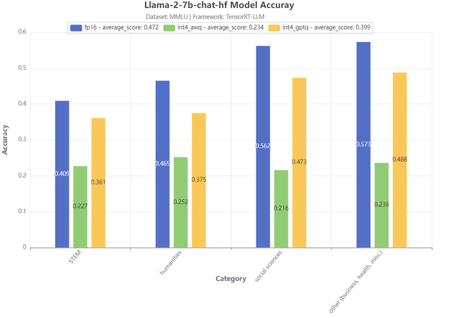
Figure 2:MMLU 4-category accuracy test result
Figure 2 shows the accuracy test results of 4 main MMLU categories for the Llama-2-7b-chat-hf model. Compared to the baseline fp16 model, we can see that the model with 4-bit AWQ has a significant accuracy drop. On the other hand, the model with 4-bit GPTQ has a much smaller accuracy drop, especially for the STEM category, the accuracy drop is smaller than 5%.
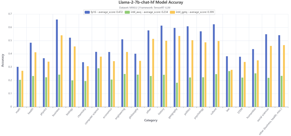
Figure 3:MMLU 21-category accuracy test result
Figure 3 further shows the accuracy test results of 21 MMLU sub-categories for the Llama-2-7b-chat-hf model. Similar conclusions can be made that the 4-bit GPTQ quantization gives much better accuracy, except for the law category, the two quantization techniques achieve a close accuracy.
Performance
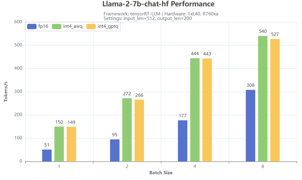
Figure 4: Throughput test result
Figure 4 shows the throughput numbers when running Llama-2-7b-chat-hf with different batch size and quantization methods on R760xa server. We observe significant throughput boost with the 4-bit quantization, especially when the batch size is small. For example, a 3x tokens/s is achieved when the batch size is 1 when comparing the scenarios with 4-bit AWQ or GPTQ quantization to the 16-bit baseline scenario. Both AWQ and GPTQ quantization give similar performance across different batch sizes.
GPU Memory Usage
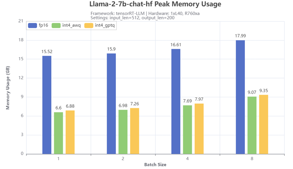
Figure 5: Peak GPU memory usage
Figure 5 shows the peak GPU memory usage when running Llama-2-7b-chat-hf with different batch size and quantization methods on R760xa server. From the results, 4-bit quantization techniques greatly reduced the memory required for running the model. Compared to the memory size required for the baseline fp16 model, the quantized models with AWQ or GPTQ only requires half or even less of the memory, depending on the batch size. A slightly larger peak memory usage is also observed for GPTQ quantized model compared to the AWQ quantized model.
Conclusion
- We have shown the impacts for accuracy, performance, and GPU memory usage by applying advanced 4-bit quantization techniques on Dell PowerEdge server when running Llama 7B model.
- We have demonstrated the great benefits of these 4-bit quantization techniques in terms of improving throughput and saving GPU memory.
- We have quantitively compared the quantized models with the baseline model in terms of accuracy among various subjects based on the MMLU dataset.
- Tests showed that with an acceptable accuracy loss, 4-bit GPTQ is an attractive quantization method for the LLM deployment where the hardware resource is limited. On the other hand, large accuracy drops across many MMLU subjects have been observed for the 4-bit AWQ. This indicates the model should be limited to the applications tied to some specific subjects. Otherwise, other techniques like re-training or fine-turning techniques may be required to improve accuracy.
References
[1]. A. Vaswani et. al, “Attention Is All You Need”, https://arxiv.org/abs/1706.03762
[2]. https://huggingface.co/meta-llama/Llama-2-7b-chat-hf
[4]. https://www.nvidia.com/en-us/data-center/l40/
[5]. https://github.com/NVIDIA/TensorRT-LLM
[7]. J. Lin et. al, “AWQ: Activation-aware Weight Quantization for LLM Compression and Acceleration”, https://arxiv.org/abs/2306.00978
[8]. E. Frantar et. al, “GPTQ: Accurate Post-Training Quantization for Generative Pre-trained Transformers”, https://arxiv.org/abs/2210.17323
[9]. D. Hendrycks et. all, “Measuring Massive Multitask Language Understanding”, https://arxiv.org/abs/2009.03300
[10]. https://github.com/hendrycks/test/blob/master/categories.py

MLPerf™ Inference 3.1 on Dell PowerEdge Server with Intel® 4th Generation Xeon® CPU
Thu, 11 Jan 2024 19:43:07 -0000
|Read Time: 0 minutes
Introduction
MLCommons™ has released the v3.1 results for its machine learning inference benchmark suite, MLPerf™. This blog focuses on the impressive datacenter inference results obtained across different use cases by using the new 4th Generation Intel Xeon Scalable Processors on a Dell PowerEdge R760 server. This submission covers the benchmark results for all 7 use cases defined in MLPerf™, which are Natural Language Processing (BERT), Image Classification (ResNet50), Object Detection (RetinaNet), Speech-to-Text (RNN-T), Medical Imaging (3D-Unet), Recommendation Systems (DLRMv2), and Summarization (GPT-J).
These new Intel® Xeon® processors use an Intel AMX® matrix multiplication engine in each core to boost overall inferencing performance. With a focus on ease of use, Dell Technologies delivers exceptional CPU performance results out of the box with an optimized BIOS profile that fully unleashes the power of Intel’s OneDNN software – software which is fully integrated with both PyTorch and TensorFlow frameworks. The server configurations and the CPU specifications in the benchmark experiments are shown in Tables 1 and 2 respectively.
System Name | PowerEdge R760 |
Status | Available |
System Type | Data Center |
Number of Nodes | 1 |
Host Processor Model | 4th Generation Intel® Xeon® Scalable Processors |
Host Processors per Node | 2 |
Host Processor Core Count | 56 |
Host Processor Frequency | 2.0 GHz, 3.8 GHz Turbo Boost |
Host Memory Capacity | 1TB, 16 x 64GB DIMM 4800 MHz |
Host Storage Capacity | 4.8 TB, NVME |
Table 1. Dell PowerEdge R760 Server Configuration
Product Collection | 4th Generation Intel® Xeon® Scalable Processors |
Processor Name | Platinum 8480+ |
Status | Launched |
# of CPU Cores | 56 |
# of Threads | 112 |
Base Frequency | 2.0 GHz |
Max Turbo Speed | 3.8 GHz |
Cache L3 | 105 MB |
Memory Type | DDR5 4800 MT/s |
ECC Memory Supported | Yes |
Table 2. 4th Generation Intel® Xeon® Scalable Processor Technical Specifications
MLPerf™ Inference v3.1 - Datacenter
The MLPerf™ inference benchmark measures how fast a system can perform ML inference using a trained model with new data in a variety of deployment scenarios. There are two benchmark suites – one for Datacenter systems and one for Edge. Table 3 lists the 7 mature models with each targeting a different task in the official release v3.1 for Datacenter systems category that were run on this PowerEdge R760. Compared to the v3.0 release, v3.1 added the updated version of the recommendation model – DLRMv2 – and introduced the first Large-Language Model (LLM) – GPT-J.
Area | Task | Model | Dataset | QSL Size | Quality | Server latency constraint |
Vision | Image classification | ResNet50-v1.5 | ImageNet (224x224) | 1024 | 99% of FP32 (76.46%) | 15 ms |
Vision | Object detection | RetinaNet | OpenImages (800x800) | 64 | 99% of FP32 (0.20 mAP) | 100 ms |
Vision | Medical imaging | 3D-Unet | KITS 2019 (602x512x512) | 16 | 99.9% of FP32 (0.86330 mean DICE score) | N/A |
Speech | Speech-to-text | RNN-T | Librispeech dev-clean (samples < 15 seconds) | 2513 | 99% of FP32 (1 - WER, where WER=7.452253714852645%) | 1000 ms |
Language | Language processing | BERT-large | SQuAD v1.1 (max_seq_len=384) | 10833 | 99% of FP32 and 99.9% of FP32 (f1_score=90.874%) | 130 ms |
Language | Summarization | GPT-J-99 | CNN Dailymail (v3.0.0, max_seq_len=2048) | 13368 | 99% of FP32 (f1_score=80.25% rouge1=42.9865, rouge2=20.1235, rougeL=29.9881). | 20 s |
Commerce | Recommendation | DLRMv2 | Criteo 4TB Multi-hot | 204800 | 99% of FP32 (AUC=80.25%) | 60 ms |
Table 3. Datacenter Suite Benchmarks. Source: MLCommons™
Scenarios
The models are deployed in a variety of critical inference applications or use cases known as “scenarios” where each scenario requires different metrics, demonstrating production environment performance in practice. Following is the description of each scenario. Table 4 shows the scenarios required for each Datacenter benchmark included in this submission v3.1.
Offline scenario: represents applications that process the input in batches of data available immediately and do not have latency constraints for the metric performance measured in samples per second.
Server scenario: represents deployment of online applications with random input queries. The metric performance is measured in queries per second (QPS) subject to latency bound. The server scenario is more complicated in terms of latency constraints and input queries generation. This complexity is reflected in the throughput-degradation results compared to the offline scenario.
Each Datacenter benchmark requires the following scenarios:
Area | Task | Required Scenarios |
Vision | Image classification | Server, Offline |
Vision | Object detection | Server, Offline |
Vision | Medical imaging | Offline |
Speech | Speech-to-text | Server, Offline |
Language | Language processing | Server, Offline |
Language | Summarization | Server, Offline |
Commerce | Recommendation | Server, Offline |
Table 4. Datacenter Suite Benchmark Scenarios. Source: MLCommons™
Software stack and system configuration
The software stack and system configuration used for this submission is summarized in Table 5.
OS | CentOS Stream 8 (GNU/Linux x86_64) |
Intel® Optimized Inference SW for MLPerf™ | MLPerf™ Intel OneDNN integrated with PyTorch |
ECC memory mode | ON |
Host memory configuration | 1TiB |
Turbo mode | ON |
CPU frequency governor | Performance |
Table 5. System Configuration
What is Intel AMX (Advanced Matrix Extensions)?
Intel AMX is a built-in accelerator that enables 4th Gen Intel Xeon Scalable processors to optimize deep learning (DL) training and inferencing workloads. With the high-speed matrix multiplications enabled by Intel AMX, 4th Gen Intel Xeon Scalable processors can quickly pivot between optimizing general computing and AI workloads.
Imagine an automobile that could excel at city driving and then quickly shift to deliver Formula 1 racing performance. 4th Gen Intel Xeon Scalable processors deliver this level of flexibility. Developers can code AI functionality to take advantage of the Intel AMX instruction set as well as code non-AI functionality to use the processor instruction set architecture (ISA).
Intel has integrated the Intel® oneAPI Deep Neural Network Library (oneDNN) – its oneAPI DL engine – into popular open-source tools for AI applications, including TensorFlow, PyTorch, PaddlePaddle, and ONNX.
AMX architecture
Intel AMX architecture consists of two components, as shown in Figure 1:
- Tiles consist of eight two-dimensional registers, each 1 kilobyte in size. They store large chunks of data.
- Tile Matrix Multiplication (TMUL) is an accelerator engine attached to the tiles that performs matrix-multiply computations for AI.

Figure 1. Intel AMX architecture consists of 2D register files (tiles) and TMUL
Results
Both MLPerf™ v3.0 and MLPerf™ v3.1 benchmark results are based on the latest Dell R760 server utilizing 4th Generation Intel® Xeon® Scalable Processors.
For the ResNet50 Image Classification, RetinaNet Object Detection, BERT Large Language, and RNN-T Speech Models – which are identical models with same datasets for both MLPerf™ v3.0 and MLPerf™ v3.1 – we re-run those for the latest submission. The results show negligible differences between two submissions.
We added three new benchmark results for MLPerf™ v3.1 submission compared to MLPerf™ v3.0 submission. Those are 3D-Unet Medical Imaging, DLRMv2 Recommendation, and GPT-J Summarization models. Given that there is no previous result for comparison, we simply show the current result on the R760.
Comparing Performance from MLPerfTM v3.1 to MLPerfTM v3.0
ResNet50 server & offline scenarios:
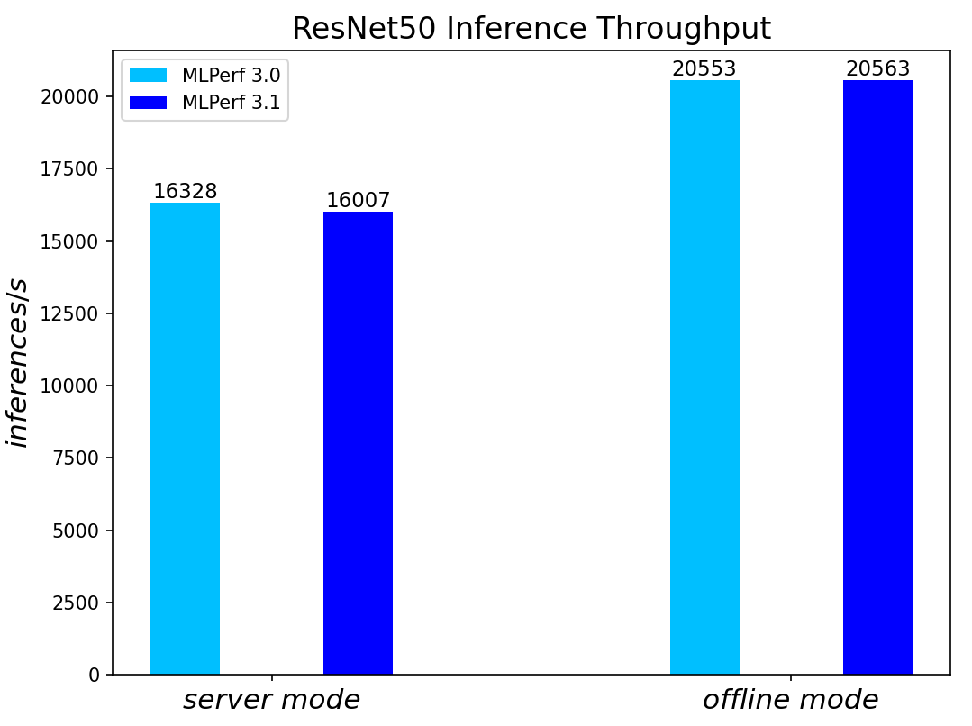
Figure 2. ResNet50 inference throughput in server and offline scenarios
BERT Large Language Model server & offline scenarios:
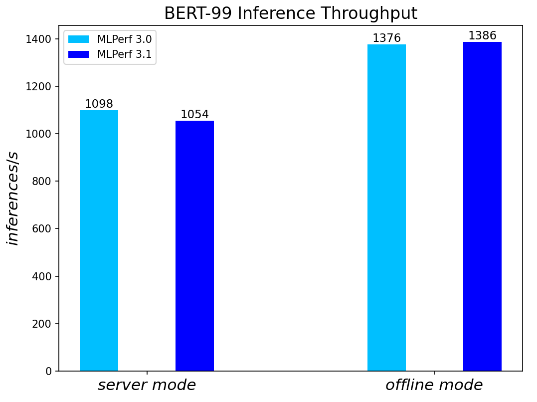
Figure 3. BERT Inference results for server and offline scenarios
RetinaNet Object Detection Model server & offline scenarios:
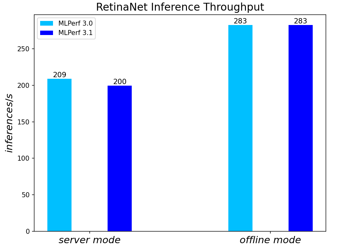
Figure 4. RetinaNet Object Detection Model Inference results for server and offline scenarios
RNN-T Text to Speech Model server & offline scenarios:
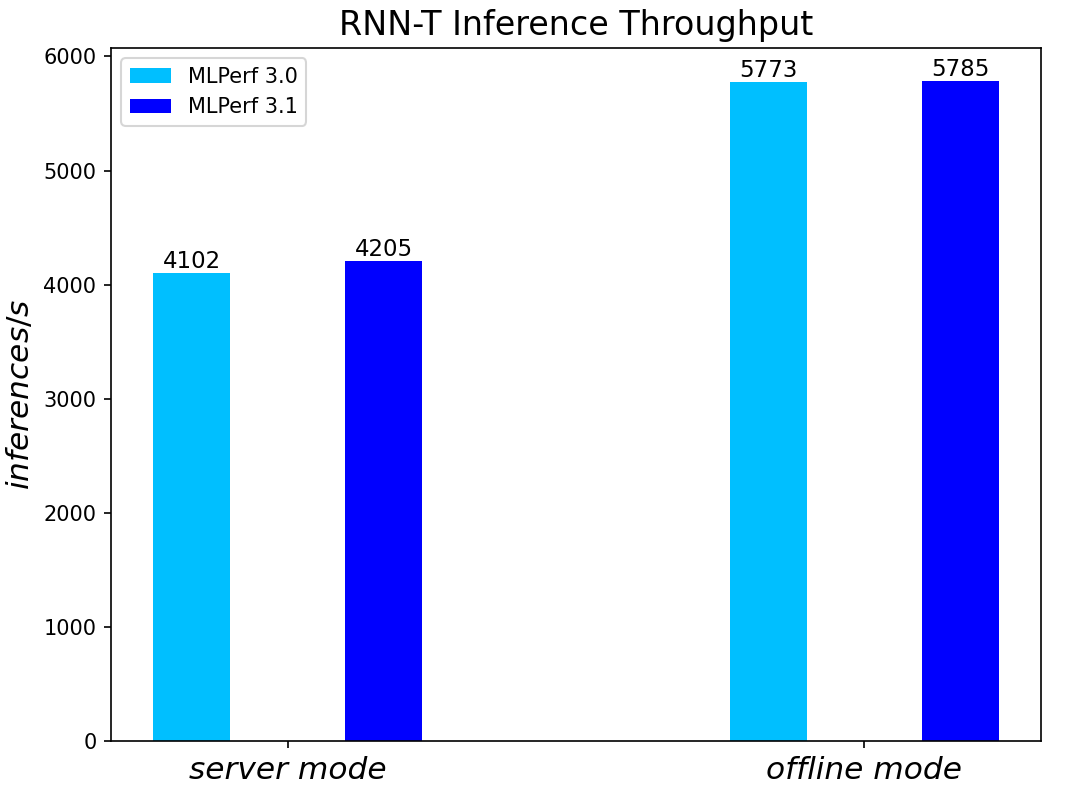
Figure 5. RNN-T Text to Speech Model Inference results for server and offline scenarios
3D-Unet Medical Imaging Model offline scenarios:
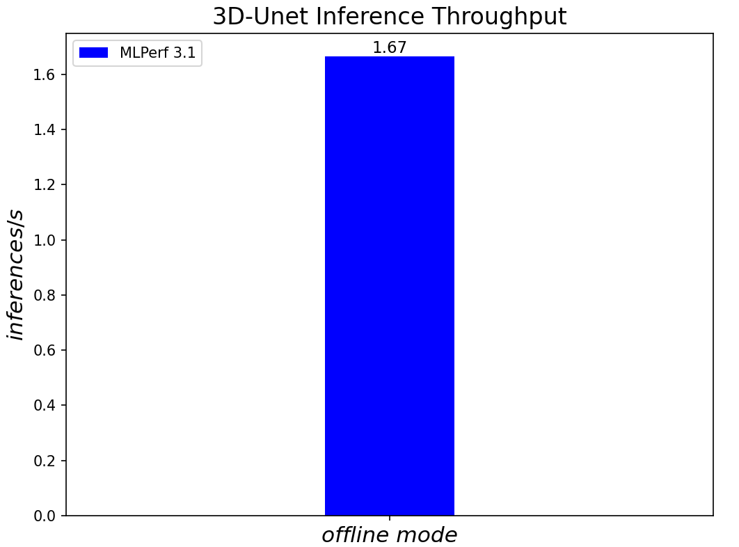
Figure 6. 3D-Unet Medical Imaging Model Inferencing results for server and offline scenarios
DLRMv2-99 Recommendation Model server & offline scenarios:
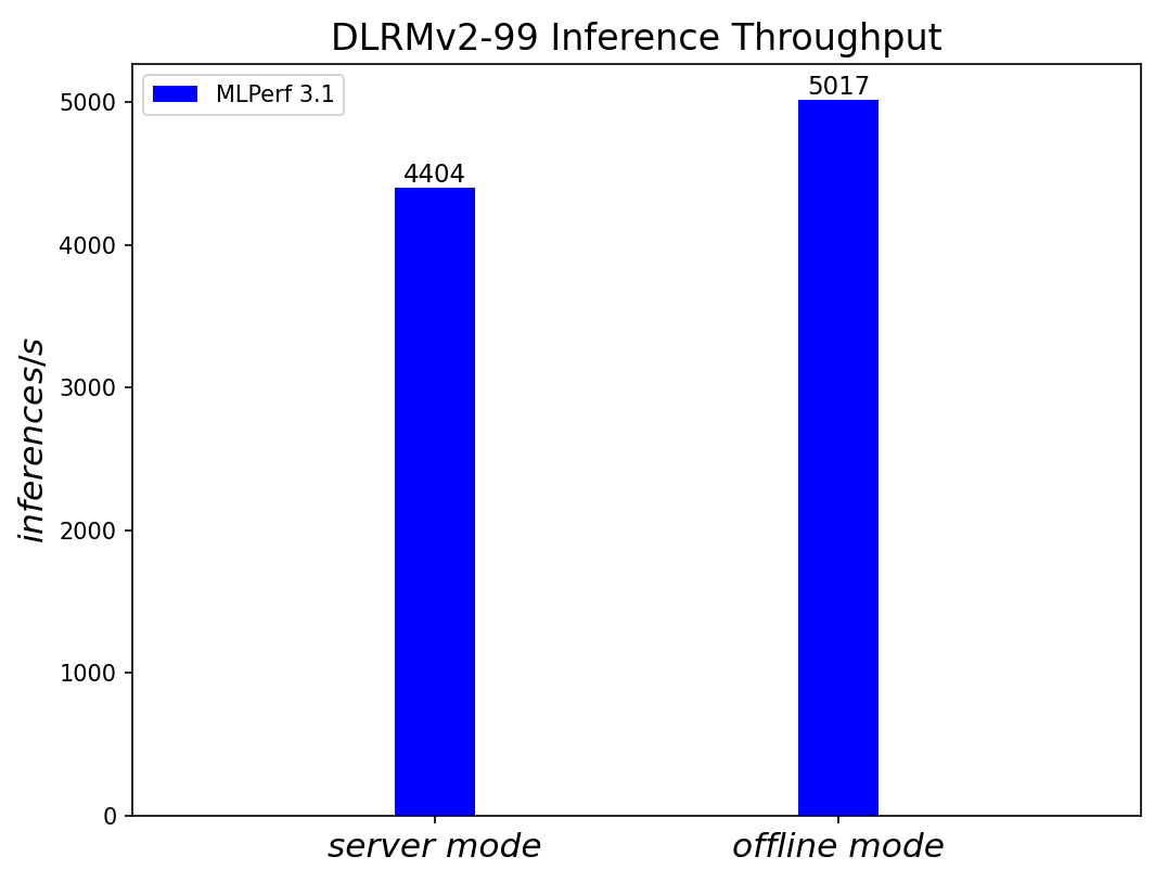
Figure 7. DLRMv2-99 Recommendation Model Inference results for server and offline scenarios (submitted in the open category)
GPT-J-99 Summarization Model server & offline scenarios:
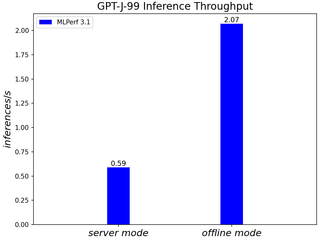
Figure 8. GPT-J-99 Summarization Model Inference results for server and offline scenarios
Conclusion
- The PowerEdge R760 server with 4th Generation Intel® Xeon® Scalable Processors produces strong data center inference performance, confirmed by the official version 3.1 MLPerfTM benchmarking results from MLCommonsTM.
- The high performance and versatility are demonstrated across natural language processing, image classification, object detection, medical imaging, speech-to-text inference, recommendation, and summarization systems.
- The R760 with 4th Generation Intel® Xeon® Scalable Processors show good performance in supporting generative AI models like GPT-J.
- The R760 supports different deep learning inference scenarios in the MLPerfTM benchmark scenarios as well as other complex workloads such as database and advanced analytics. It is an ideal solution for data center modernization to drive operational efficiency, lead higher productivity, and minimize total cost of ownership (TCO).
References
MLCommonsTM MLPerfTM v3.1 Inference Benchmark Submission IDs
ID | Submitter | System |
3.1-0059 | Dell | Dell PowerEdge Server R760 (1x Intel Xeon Platinum 8480+) |
3.1-0060 | Dell | Dell PowerEdge Server R760 (1x Intel Xeon Platinum 8480+) |
3.1-4184 | Dell | Dell PowerEdge Server R760 (1x Intel Xeon Platinum 8480+) |
Authors: Tao Zhang (tao.zhang9@dell.com); Brandt Springman (brandt.springman@dell.com); Bhavesh Patel (bhavesh_a_patel@dell.com); Louie Tsai (louie.tsai@intel.com); Yuning Qiu (yuning.qiu@intel.com); Ramesh Chukka (ramesh.n.chukka@intel.com)

Running LLMs on Dell PowerEdge Servers with Intel® 4th Generation Xeon® CPUs
Thu, 11 Jan 2024 19:38:53 -0000
|Read Time: 0 minutes
Introduction
Large-language Models (LLMs) have gained great industrial and academic interests in recent years. Different LLMs have been adopted in various applications, such as content generation, text summarization, sentiment analysis, and healthcare. The list goes on.
When we think about LLMs and what methodologies we can use for inferencing and fine-tuning, the question always comes up as to which compute device we should use. For inferencing, we wanted to explore what the performance metrics are when running on an Intel 4th Generation CPU, and what are some of the variables we should explore?
This blog focuses on LLM inference results on Dell PowerEdge Servers with the 4th Generation Intel® Xeon® Scalable Processors. Specifically, we demonstrated their performance and power while running the stable diffusion and Llama2 chat models on R760 and HS5610 servers. We also explored the performance and power impacts with different quantization bits and CPU/socket numbers through experiments and will present the inference results of stable diffusion and Llama2 models obtained on a Dell PowerEdge R760 and HS5610 with the 4th Generation Intel® Xeon® Scalable Processors.
We selected the aforementioned Dell platforms because we wanted to explore how our CSP-focused platforms like HS5610 perform when it comes to inferencing and whether they can meet the requirements for LLM models. These new Intel® Xeon® processors use an Intel AMX® matrix multiplication engine in each core to boost overall inferencing performance. By combining with the quantization techniques, we further improved the inference performance with the CPU-only system. Moreover, we also show how the CPU core and socket numbers affect the performance results.
Background
Transformer is regarded as the 4th fundamental model after Multilayer Perceptron (MLP), Recurrent Neural Networks (RNN), and Convolutional Neural Networks (CNN). Known for its parallelization and scalability, transformer has greatly boosted the performance and capability of LLMs since it was introduced in 2017 [1].
Today, LLMs have been rapidly adopted in various applications like content generation, text summarization, sentiment analysis, code generation, healthcare, and so on, as shown in Figure 1 [2]. This trend is continuing. More open-source LLMs are popping up almost on a monthly basis. Moreover, the transformer-based techniques are being used alongside with other methods, greatly improving the accuracy and performance of the original tasks. For example, the stable diffusion model uses the LLM at the input as the neural language understanding engine. Combined with the diffusion model, it has greatly improved the quality and throughput of the text-to-image generation task [3]. Note that for simplicity in this blog, we use the term “LLMs” to represent both those transformer-based models shown in Figure 1 and the derivative models like stable diffusion models.
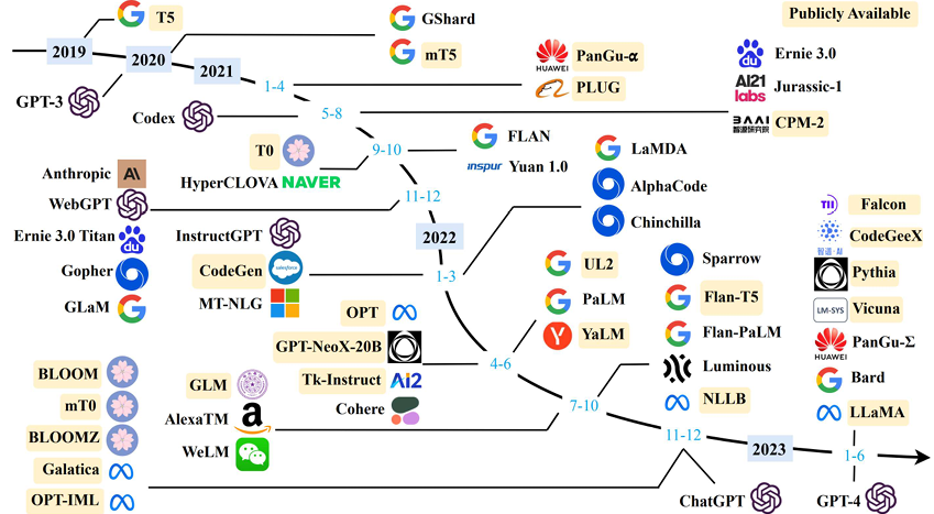
Figure 1. LLM Timeline [2] Image credit: Wayne Xin Zhao, et.al, “A Survey of Large Language Models”]
While training and fine-tuning those LLMs is normally time- and cost-consuming, deploying the LLMs at the edge has its own challenges. Considering both performance and power, deploying the LLMs can be, in a sense, more cost-sensitive given the volumes of the systems required to cover various applications. GPUs are widely used to deploy LLMs. In this blog, we demonstrate the feasibility of deploying those LLMs with Intel 4th generation Intel® Xeon® CPUs with Dell PowerEdge servers and illustrate that good performance can be achieved with a proper hardware configuration – like CPU core numbers and quantization method for popular LLMs.
Test Setup
The hardware platforms we used for the experiments are PowerEdge R760 and HS5610, which are the latest mainstream and cloud-optimized servers respectively from Dell product portfolio. Figure 2 shows the rack-level interface for the HS5610 server. As a cloud-optimized solution, the HS5610 server has been designed with CSP features that allow the same benefits with full PowerEdge features and management like the mainstream server R760, as well as open management (OpenBMC), cold aisle service, channel firmware, and services. Both servers have two sockets with an Intel 4th generation Xeon CPU on each socket. R760 features a 56-core CPU – Intel® Xeon® Platinum 8480+ (TDP: 350W) in each socket, and HS5610 has a 32-core CPU – Intel® Xeon® Gold 6430 (TDP: 250W) in each socket. Tables 1-4 show the details of the server configurations and CPU specifications. During tests, we use the numactl command to set the numbers of the sockets or CPU cores to execute the LLM inference tasks.
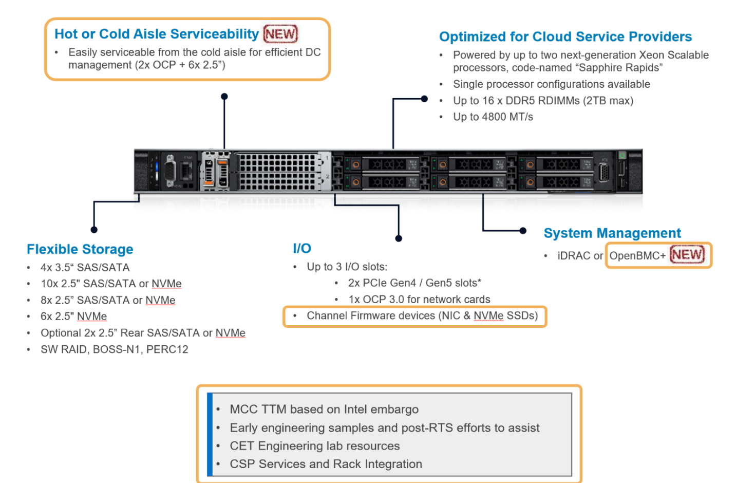
Figure 2. PowerEdge HS5610 [4]
System Name | PowerEdge R760 |
Status | Available |
System Type | Data Center |
Number of Nodes | 1 |
Host Processor Model | 4th Generation Intel® Xeon® Scalable Processors |
Host Processors per Node | 2 |
Host Processor Core Count | 56 |
Host Processor Frequency | 2.0 GHz, 3.8 GHz Turbo Boost |
Host Memory Capacity | 1TB, 16 x 64GB DIMM 4800 MHz |
Host Storage Capacity | 4.8 TB, NVME |
Table 1. R760 Server Configuration
Product Collection | 4th Generation Intel® Xeon® Scalable Processors |
Processor Name | Platinum 8480+ |
Status | Launched |
# of CPU Cores | 56 |
# of Threads | 112 |
Base Frequency | 2.0 GHz |
Max Turbo Speed | 3.8 GHz |
Cache L3 | 108 MB |
Memory Type | DDR5 4800 MT/s |
ECC Memory Supported | Yes |
Table 2. 4th Generation 56-core Intel® Xeon® Scalable Processor Technical Specifications
System Name | PowerEdge HS5610 |
Status | Available |
System Type | Data Center |
Number of Nodes | 1 |
Host Processor Model | 4th Generation Intel® Xeon® Scalable Processors |
Host Processors per Node | 2 |
Host Processor Core Count | 32 |
Host Processor Frequency | 2.0 GHz, 3.8 GHz Turbo Boost |
Host Memory Capacity | 1TB, 16 x 64GB DIMM 4800 MHz |
Host Storage Capacity | 4.8 TB, NVME |
Table 3. HS5610 Server Configuration
Product Collection | 4th Generation Intel® Xeon® Scalable Processors |
Processor Name | Gold 6430 |
Status | Launched |
# of CPU Cores | 32 |
# of Threads | 64 |
Base Frequency | 2.0 GHz |
Max Turbo Speed | 3.8 GHz |
Cache L3 | 64 MB |
Memory Type | DDR5 4800 MT/s |
ECC Memory Supported | Yes |
Table 4. 4th Generation 32-core Intel® Xeon® Scalable Processor Technical Specifications
Software stack and system configuration
The software stack and system configuration used for this submission is summarized in Table 5. Optimizations have been done for the PyTorch framework and Transformers library to unleash the Xeon CPU machine learning capabilities. Moreover, a low-level tool -- Intel® Neural Compressor -- has been used for high-accuracy quantization.
OS | CentOS Stream 8 (GNU/Linux x86_64) |
Intel® Optimized Inference SW | OneDNN™ Deep Learning, ONNX, Intel® Extension for PyTorch (IPEX), Intel® Extension for Transformers (ITREX), Intel® Neural Compressor |
ECC memory mode | ON |
Host memory configuration | 1TiB |
Turbo mode | ON |
CPU frequency governor | Performance |
Table 5. Software stack and system configuration
The models under testing are stable diffusion model version 1.4 (~1 billion parameters) and Llama2-chat-HF models with 7 billion, 13 billion, and 70 billion parameters. We purposely choose those models because they are open-sourced, representative, and cover a wide parameter range. Different quantization bits are tested to characterize the corresponding performance and power consumption.
All the experiments are based on batch-size equal to 1. Performance is characterized by latency or throughput. To reduce the measurement errors, the inference is executed 10 times to get the averaged value. A warm-up process is executed by loading the parameter and running a sample test before running the defined inference.
Results
We show some typical results in this section alongside brief discussions for each result. The conclusions are summarized in the next section.
HS5610 Results
Latency vs Quantization vs Cores – Stable Diffusion Model:
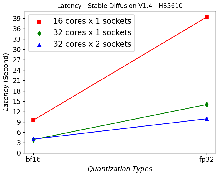
Figure 3. Latency in HS5610 server running Stable Diffusion
Figure 3 shows that HS5610 can generate a new image in approximately 3 seconds when running at bf16 Stable Diffusion V1.4 model. Quantizing to 16 bits greatly reduces the latency compared to using fp32 model. Scaling up the core numbers from 16 to 32 cores greatly reduces the latency, however scaling up across the sockets does not help. This is mainly due to the NUMA remote memory bottleneck.
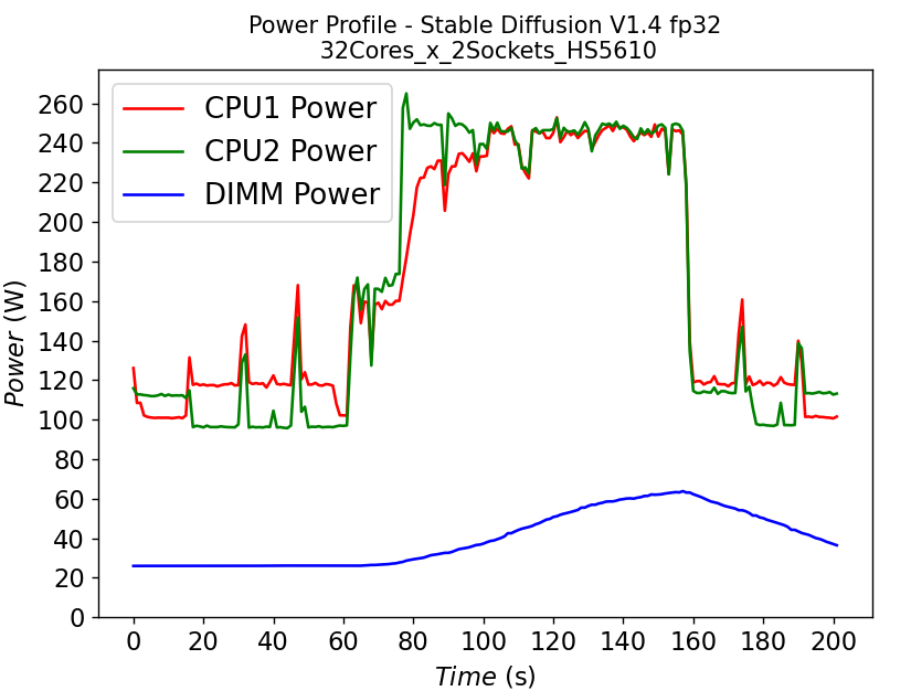
Power Consumption – Stable Diffusion Model:
 (a)
(a) 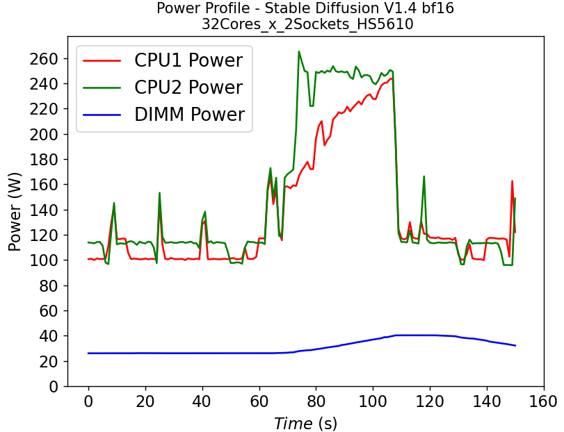 (b)
(b)
Figure 4. Power consumption of CPU and DIMM in HS5610 server running stable diffusion: (a) fp32 model (b) bf16 model
Figure 4 shows the power profile comparison of HS5610 when running the stable diffusion model with (a) fp32 weights and (b) bf16 weights. To finish the same tasks (warm up and inferencing), the bf16 model takes significantly less time (shorter power profile duration) compared to fp32 scenario. The plot also shows that much larger DIMM power is required to run fp32 compared to bf16. Executing the task pushes the CPU working close to the TDP limit, with the exception of the CPU1 in Figure 4b, indicating that further improvement is possible to further reduce the latency for the bf16 model.
Throughput vs Quantization vs Cores – Llama2 Chat Models:
 (a)
(a)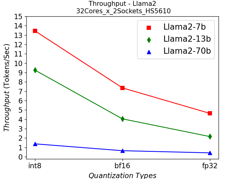 (b)
(b)
Figure 5. Throughput in HS5610 server running Llama2: (a) 1-socket (b) 2-socket
Figure 5 shows the throughput numbers when running Llama2 chat models with different parameter sizes and quantization bits in HS5610 server. Figure 5a shows the single socket scenario and 5b shows the dual-socket scenario. Smaller models with lower quantization bits give higher throughputs which is to be expected. Like the stable diffusion model, quantization greatly improves the throughput. However, scaling up with more CPU cores across the socket has negligible results in boosting the performance.
R760 Results
Throughput vs Quantization vs Cores – Llama2 Chat Models:
 (a)
(a)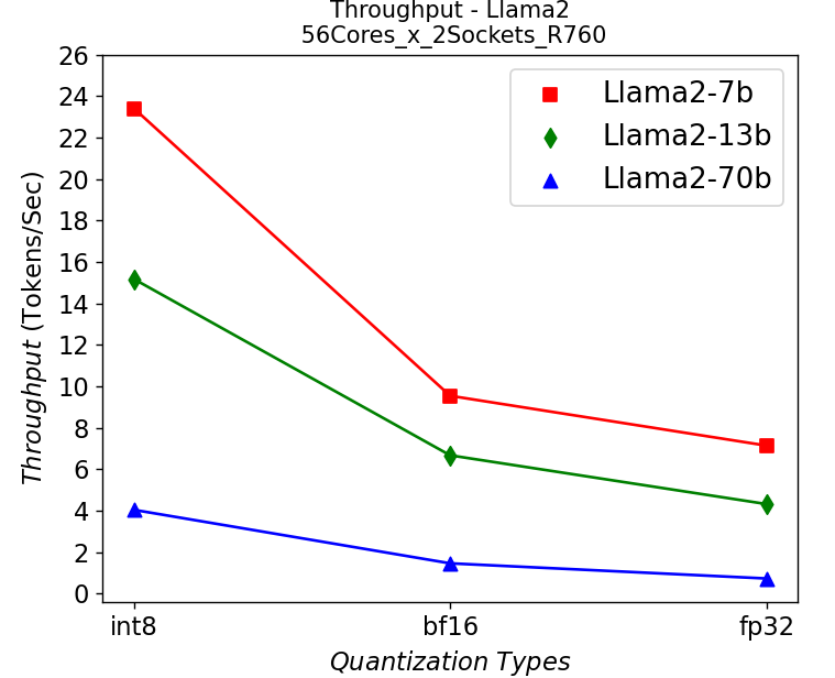 (b)
(b)
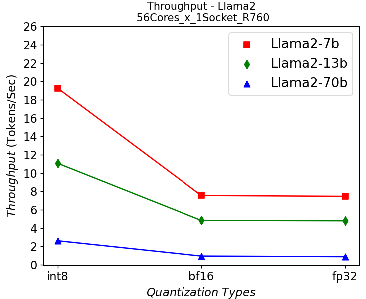
Figure 6. Throughput in R760 server running Llama2: (a) 1-socket (b) 2-socket
Figure 6 shows the throughput numbers when running Llama2 chat models with different parameter sizes and quantization bits in R760 server. We get similar observations as the results shown in HS5610 server. A smaller model gives a higher throughput, and quantization greatly improves the throughput. One difference is that we get a 10-30% performance improvement depending on models when scaling up across sockets, showing a benefit from larger core numbers. The performance across the models is good enough for most real-time chatbot applications.
Performance Per Watt – Llama2 Chat Models:
 (a)
(a)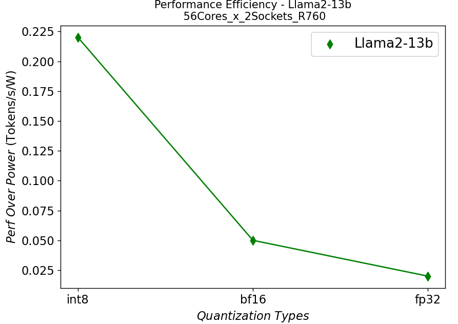 (b)
(b)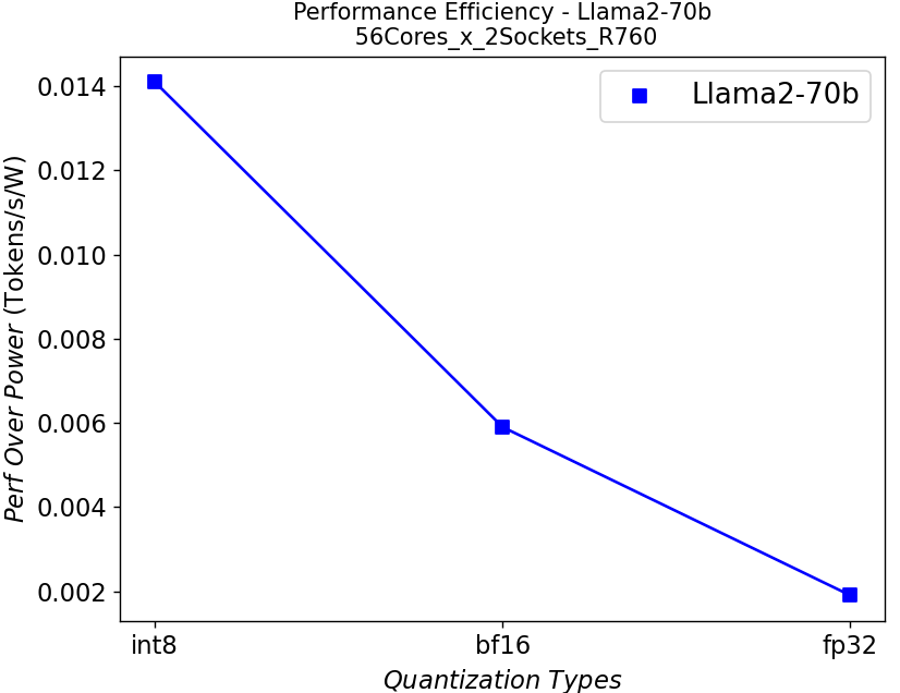 (c)
(c)
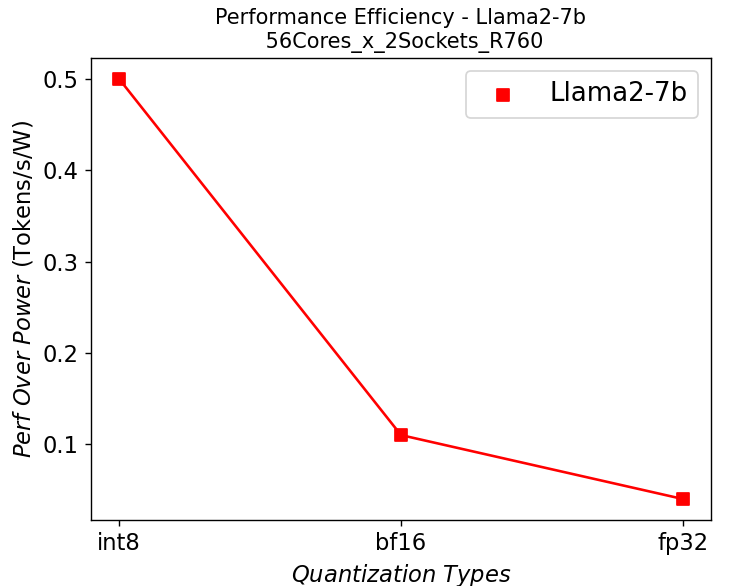
Figure 7. Performance per watt in R760 server running Llama2: (a) 7b (b)13b (c) 70b
We further plot the performance per watt curve which is strongly related to the total cost of ownership (TCO) of the system in Figure 7. From the plots, the quantization can greatly help with the performance efficiency, especially for the models with large parameters.
Conclusion
- We have shown that the Intel 4th generation Intel® Xeon® CPUs on Dell PowerEdge mainstream and HS class platforms can easily meet performance requirements when it comes to Inferencing with Llama2 models.
- We also demonstrate the benefits of quantization or using lower precision for inferencing quantitively, which can give a better TCO in terms of performance per watt and memory footprint as well as enable better user experience by improving the throughput.
- These studies also show that we need to right-size the infrastructure based on the application and model size.
References
[1]. A. Vaswani et. al, “Attention Is All You Need”, https://arxiv.org/abs/1706.03762
[2]. W. Zhao et. al, “A Survey of Large Language Models”, https://doi.org/10.48550/arXiv.2303.18223
[3]. R. Rombach et. al, “High-Resolution Image Synthesis with Latent Diffusion Models”, https://arxiv.org/abs/2112.10752
[4]. https://www.dell.com/en-us/shop/ipovw/poweredge-hs5610
Authors: Tao Zhang (tao.zhang9@dell.com); Bhavesh Patel (bhavesh_a_patel@dell.com)

Scaling Hardware and Computation for Practical Deep Learning Applications in Healthcare
Fri, 01 Dec 2023 15:26:29 -0000
|Read Time: 0 minutes
Medical practice requires analysis of large volumes of data spanning multiple modalities. While these can be as simple as numeric lab results, at the other extreme are high-complexity data such as magnetic resonance imaging or decades-worth of text-based clinical documentation which may be present in medical records. Oftentimes, small details buried within piles of clinical information are critical to obtaining a complete clinical picture. Many deep learning methods developed in recent years have focused on very short “sequence lengths” – the term used to describe the number of words or pixels that a model can ingest – of images and text compared to those encountered in clinical practice. How do we scale such tools to model this breadth of clinical data appropriately and efficiently?
In the following blog, we discuss ways to tackle the compute requirements of developing transformer-based deep learning tools for healthcare data from the hardware, data processing, and modeling perspectives. To do so, we present a practical application of Flash Attention using a series of experiments performing an analysis of the publicly available Kaggle RSNA Screening Mammography Breast Cancer Detection challenge, which contains 54,706 images of 11,913 patients. Breast cancer affects 1 in 8 women and is the second leading cause of cancer death. As such, screening mammography is one of the most performed imaging-based medical screening procedures, which offers a clinically relevant and data-centric case study to consider.
Data Primer
To detect breast cancer early when treatments are most effective, high-resolution x-ray images are taken of breast tissue to identify areas of abnormality which require further examination by biopsy or more detailed imaging. Typically, two views are acquired:
- Craniocaudal (CC) – taken from the head-to-toe perspective
- Mediolateral oblique (MLO) – taken at an angle
The dataset contains DICOM-formatted images which must be pre-processed in a standard fashion prior to model training. We detail the data preparation pipeline in figure 1. The CC and MLO views of each study are identified, flipped horizontally if necessary, cropped, and combined to form the model input image. We wrap the standard PyTorch Dataset class to load images and preprocess them for training.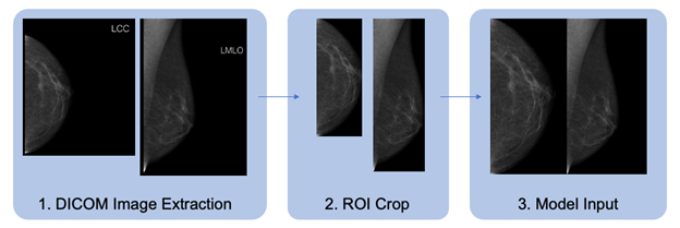 Figure 1. Data pre-processing pipeline for DICOM-formatted image
A more in-depth look at the system for data pre-processing is as follows:
- For each breast with a corresponding cancer label, the CC and MLO views are extracted, and the image data are normalized. Right-sided images are horizontally flipped so that the tissue is to the left side of the image, as shown.
- Images are cropped to the region of interest (ROI), excluding areas of black or non-tissue artifacts.
- Images are resized, maintaining aspect ratio, and tiled to a square of the output size of interest, with the CC view occupying the left half of the output and the MLO view occupying the right.
An important consideration is whether to perform this processing within the dataloader while training or to save a pre-processed version of the dataset. The former approach allows for iteration on different processing strategies without modifying the dataset itself, providing greater ease of experimentation. However, this level of processing during training may limit the rate at which data can be fed to the graphics processing unit (GPU) for training, resulting in time and monetary inefficiencies. In contrast, the latter approach requires that multiple versions of the dataset be saved locally, which is potentially prohibitive when working with large dataset sizes and storage space and/or network limitations. For the purpose of this blog post, to benchmark GPU hardware and training optimizations, we use the second method, saving data on local solid state drives connected via NVMe to ensure GPU saturation despite processor differences. In general, before implementing the training optimizations described below, it is important to first ensure that dataloading does not bottleneck the overall training process.
Scaling Up
Naturally, increasing the capability and amount of compute available for model training yields direct benefits. To demonstrate the influence of hardware on run time, we present a simple 20-epoch training experiment using the same dataset on three different servers, shown in figure 2:
- Dell XE8545 with 4x NVIDIA A100-SXM4 40GB GPUs and an AMD EPYC 7763 with 64 cores
- Dell R750xa with 4x NVIDIA A100 80GB GPUs and an Intel Xeon Gold 5320 processor with 26 cores
- Dell XE9680 server with 8 NVIDIA HGX A100 80GB SXM4 GPUs and an Intel Xeon Platinum 8470 processor with 52 cores
Input data into the model shown in figure 2 were 512x512 with a patch size of 16. Batch size was 24 per GPU on the 40GB and 64 on the 80GB servers.
Parameters remain the same for each run, except that batch size has been increased to maximally utilize GPU memory on the R750xa and XE9680 compared with the XE8545. Gradient accumulation is performed to maintain a constant global batch size per model weight update for each run. We see a clear improvement in runtime as the hardware is scaled up, demonstrating how increased compute capability directly yields time savings which enables researchers to efficiently iterate on experiments and train effective models.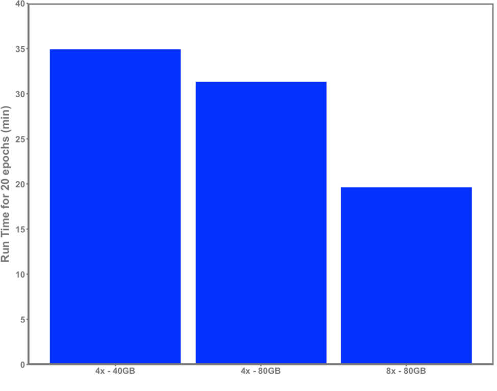 Figure 2. ViT-base training time across 20 epochs with 4xA100 40GB, 4xA100 80GB, and 8xA100 80GB servers
In conjunction with hardware, sequence lengths of data should be carefully considered given the application of interest. The selected tokenization scheme directly impacts sequence length of input data, such as the patch size selected as input to a vision transformer. For example, a patch size of 16 on a 1024x1024 image will result in a sequence length of 4,096 (Height*Width/Patch Size2) while a patch size of 8 will result in a sequence length of 16,384. While GPUs increasingly feature more memory, they present an upper bound on the sequence length that can practicably be considered. Smaller patch sizes – and thus, longer sequences – will result in slower throughput via smaller batch sizes and a greater number of computations, as shown in figure 3. However, larger images sizes coupled with smaller patch sizes are particularly relevant in analysis of mammography and other applications in which fine-resolution features are of interest.
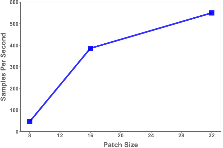 Figure 3. Average training samples per second (per GPU) for mammograms through a vision transformer by patch size
The data illustrated in figure 3 are taken from a run of twenty epochs using an image size of 512x512 and tested on an 8xA100 (80 GB) server.
Flash Attention – Experiments
Recently, Dao et al. have published on Flash Attention (https://arxiv.org/abs/2205.14135), a technique aimed at more efficiently accomplishing the computations involved within transformers via minimizing GPU high-bandwidth memory and the on-chip SRAM. Their reported findings are impressive, yielding 2-3x speedups during an attention forward and backwards pass while also having 3-20x smaller memory requirements.
Using a Dell XE9680 server with 8 NVIDIA HGX A100 80GB SXM4 GPUs and an Intel Xeon Platinum 8470 processor with 52 cores, we provide a practical demonstration of potential applications for Flash Attention and vision transformers in healthcare. Specifically, we performed experiments to demonstrate how sequence length (determined by patch size and image size) and Flash Attention impact training time. To limit confounding variables, all images were pre-sized on disk and directly loaded into the vision transformer without any permutations. For the vision transformer, the ViT-Base from Huggingface was used. For Flash Attention, the Encoder from the x_transformers library was used, shown being implemented in the following code.
All tests were carried out with the Huggingface trainer using an effective batch size of 128 per GPU, “brain" floating-point 16 data, and across twenty epochs at patch sizes of 8, 16, and 32 with image sizes of 384, 512, 1024, and 2048.
from x_transformers import ViTransformerWrapper, Encoder
class FlashViT(nn.Module):
    def __init__(self,
                 encoder = ViTransformerWrapper(
                     image_size = args.img_size,
                     patch_size = args.patch_size,
                     num_classes = 2,
                     channels=3,
                     attn_layers = Encoder(
                         dim = 768,
                         depth = 12,
                         heads = 12,
                         attn_flash=True
                         )
                     ),
    super().__init__()
    self.encoder = encoder

    def forward(self,
                pixel_values:torch.tensor,
                labels:torch.tensor):
             """
                 pixel_values: [batch,channel,ht,wt] of pixel values
                 labels: labels for each image
             """
             logits = self.encoder(pixel_values)
             return {'loss':F.cross_entropy(logits,labels),'logits':logits}
model = FlashViT()
Figure 4 demonstrates the pronounced benefit of using Flash Attention within a vision transformer with respect to model throughput. With the exception of the two smallest image sizes and largest patch size (and thus shortest sequence length), Flash Attention resulted in a marked speed increase across all other perturbations. The speed-up range across patch sizes was:
- Patch size of 8: 3.0 - 4.2x
- Patch size of 16: 2.8 – 4.0x
- Patch size of 32: 0 - 2.3x
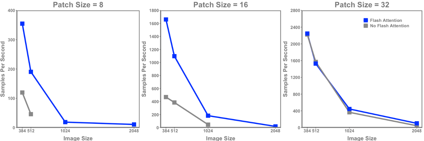 Figure 4. Samples per second throughput for a ViT-base vision transformer with and without Flash Attention across varying image sizes and patch sizes
Another benefit demonstrated in these experiments is the additional image and patch size combinations achievable only with Flash Attention due to the reduced GPU memory requirement. Non-Flash Attention models could only be used on image sizes of 2,048 if a patch size of 32 was used (sequence length of 4,096), whereas Flash Attention was capable of running on patch sizes of 8 and 16. Even at shorter sequence lengths (576 - 384x384 image, patch size of 16), there was 2.3x less memory used for Flash Attention. Use of Flash Attention will also be critical when considering larger transformer models, with ViT-Huge having more than 7x the parameters than ViT-Base. In conjunction with hardware-enabling distributed training at scale such as the Dell XE9680, these optimizations will enable new findings at unprecedented scales.
Takeaways
We have described methods by which the benefits of transformer-based models can be scaled to the longer sequences which medical data often require. Notably, we demonstrate the benefits of implementing Flash Attention to a vision encoder. Flash Attention presents marked benefit from a modeling perspective, from shorter runtimes (and thus lower cost) to better image encoding (longer sequence lengths). Moreover, we show that these benefits scale substantially along with sequence length, making them indispensable for practitioners aiming to model the full complexity of hospital data. As machine learning continues to grow in healthcare, tight collaborations between hospitals and technology manufactures are thus essential to allow for greater compute resources to input higher-quality data into machine learning models.
Resources
- Dell XE9680 Technical Guide: https://www.delltechnologies.com/asset/en-ca/products/servers/technical-support/poweredge-xe9680-technical-guide.pdf
- Dell R750xa Technical Guide: https://i.dell.com/sites/csdocuments/Product_Docs/en/poweredge-r750xa-technical-guide.pdf
- Dell XE8545 Technical Guide: https://i.dell.com/sites/csdocuments/product_docs/en/poweredge-xe8545-technical-guide.pdf
Authors:
Jonathan Huang, MD/PhD Candidate, Research & Development, Northwestern Medicine
Matthew Wittbrodt, Solutions Architect, Research & Development, Northwestern Medicine
Alex Heller, Director, Research & Development, Northwestern Medicine
Mozziyar Etemadi, Clinical Director, Advanced Technologies, Northwestern Medicine
Bhavesh Patel, Sr. Distinguished Engineer, Dell Technologies
Bala Chandrasekaran, Technical Staff, Dell Technologies
Frank Han, Senior Principal Engineer, Dell Technologies

MLPerf™ Inference v1.0 – CPU Based Benchmarks on Dell PowerEdge R750 Server
Tue, 17 Jan 2023 06:44:49 -0000
|Read Time: 0 minutes
Summary
MLCommons™ Association has released the third round of results v1.0 for its machine learning inference performance benchmark suite MLPerf™. Dell EMC has participated in this effort by collaborating with several partners and using multiple configurations, spanning from Intel® CPU to accelerators such as GPU’s and FPGA’s. This blog is focused on the results for computer vision inference benchmarks (image classification and object detection), in the closed division / datacenter category, running on Dell EMC PowerEdge R750 in collaboration with Intel® and using its Optimized Inference System based on OpenVINO™ 2021.1.
Introduction
In this blog we present the MLPerf™ Inference v1.0 CPU based results submitted on PowerEdge R750 with Intel® processor using the Intel® optimized inference system based on OpenVINO™ 2021.1. Table 1 shows the technical specifications of this system.
Dell EMC PowerEdge R750 Server
System Name | PowerEdge R750 |
Status | Coming soon |
System Type | Data Center |
Number of Nodes | 1 |
Host Processor Model Name | Intel(R) Xeon(R) Gold 6330 CPU @ 2.0GHz |
Host Processors per Node | 2 |
Host Processor Core Count | 28 |
Host Processor Frequency | 2.00 GHz |
Host Memory Capacity | 1TB 1 DPC 3200 MHz |
Host Storage Capacity | 1.5TB |
Host Storage Type | NVMe |
3rd Generation Intel® Xeon® Scalable Processor
The 3rd Generation Intel® Xeon® Scalable processor family is designed for data center modernization to drive operational efficiency and higher productivity, leveraged with built-in AI acceleration tools, to provide the seamless performance foundation for data center and edge systems. Table 2 shows the technical specifications for CPU’s Intel® Xeon®.
Product Collection | 3rd Generation Intel® Xeon® Scalable Processors |
Code Name | Ice Lake |
Processor Name | Gold 6330 |
Status | Launched |
# of CPU Cores | 28 |
# of Threads | 56 |
Processor Base Frequency | 2.0GHz |
Max Turbo Speed | 3.10GHz |
Cache L3 | 42 MB |
Memory Type | DDR4-2933 |
ECC Memory Supported | Yes |
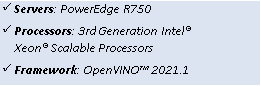
MLPerf™ Inference v1.0 - Datacenter
The MLPerf™ inference benchmark measures how fast a system can perform ML inference using a trained model with new data in a variety of deployment scenarios. There are two benchmark suites, one for Datacenter systems and one for Edge. Table 3 lists six mature models included in the official release v1.0 for Datacenter systems category and the vision models both image classification and object detection. The benchmark models highlighted below were run on PowerEdge R750.
Datacenter Benchmark Suite
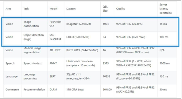
Table 3: Datacenter Suite Benchmarks. Source: MLCommons™
Scenarios
The above models are deployed in a variety of critical inference applications or use cases known as “scenarios”, where each scenario requires different metrics, demonstrating production environment performance in the real practice. Below is the description of each scenario and the Table 4 shows the scenarios required for each Datacenter benchmark included in this submission v1.0.
Offline scenario: represents applications that process the input in batches of data available immediately, and don’t have latency constraint for the metric performance measured as samples per second.
Server scenario: this scenario represents deployment of online applications with random input queries, the metric performance is queries per second (QPS) subject to latency bound. The server scenario is more complicated in terms of latency constraints and input queries generation, this complexity is reflected in the throughput-degradation results compared to offline scenario.
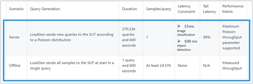
Table 4: MLPerf™ Inference Scenarios. Source: MLCommons™
Software Stack and System Configuration
The software stack and system configuration used for this submission is summarized in Table 5. Some of the settings that really mattered when looking at benchmark performance are captured in the table below.
OS | Ubuntu 20.10 (GNU/Linux 5.8.0-45-generic x86_64) |
Intel® Optimized Inference SW for MLPerf™ | MLPerf™ Intel OpenVino OMP CPP v1.0 Inference Build |
ECC memory mode | ON |
Host memory configuration | 1TiB | 64G per memory channel (1DPC) with 2933mt/s |
Turbo mode | ON |
CPU frequency governor | Performance |
OpenVINO™ Toolkit
The OpenVINO™ 2021.1 toolkit is used to optimize and run Deep Learning Neural Network models on Intel® hardware. The toolkit consists of three primary components: inference engine, model optimizer, and intermediate representation. The Model Optimizer is used to convert the MLPerf™ reference implementation benchmarks from a framework into quantized INT8 models to run on Intel® architecture.
Benchmark Parameter Configurations
The benchmarks and scenarios submitted for this round are ResNet50-v1.5 and SSD-ResNet34 in offline and server scenarios. Both benchmarks required tunning certain parameters to achieve maximum performance. The parameter configurations and expected performance depend on the processor characteristics including number on CPUs used (number of sockets), number of cores, number of threads, batch size, number of requests, CPU frequency, memory configuration and the software accelerator. Table 6 shows the parameter setting used to run the benchmarks to obtain optimal performance and produce VALID results to pass Compliance tests.
Model | Scenario | OpenVINO params & batch size |
ResNet50 INT8 | Offline | nireq = 224, nstreams = 112, nthreads = 56, batch = 4 |
Server | nireq = 28, nstreams = 14, nthreads = 56, batch = 1 | |
SSD-ResNet34 INT8 | Offline | nireq = 28, nstreams = 28, nthreads = 56, batch = 1 |
Server | nireq = 4, nstreams = 2, nthreads = 56, batch = 1 |
Results
From the scenario perspective, we benchmark the CPU performance by comparing server versus offline scenario and determine what is the delta. We also looked at results from our prior submission v0.7 to v1.0, so we can determine how the performance improved for Intel Xeon 3rd Generation compared to Intel Xeon 2nd.
ResNet50-v1.5 in server and offline scenarios
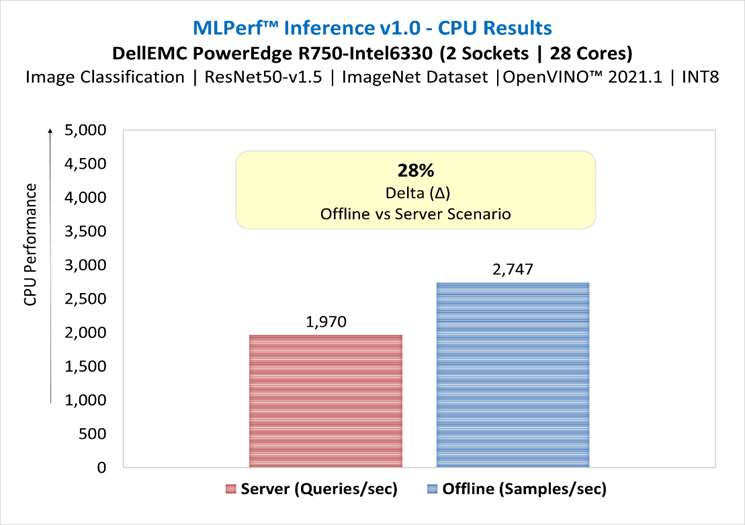
Figure 1: ResNet50-v1.5 in server and offline scenarios
SSD-ResNet34 in server and offline scenarios
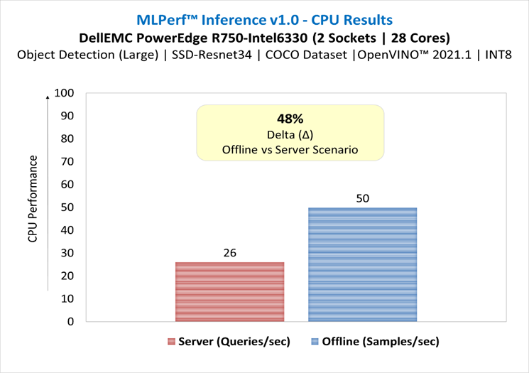
Figure 2: SSD-ResNet34 in server and offline scenario
Figure 3 illustrates the normalized server-to-offline performance for each model, scores close to 1 indicate that the model is delivering similar throughput in server scenario (constrained latency) as it is in offline scenario (unconstrained latency), scores close to zero indicate severe throughput degradation.
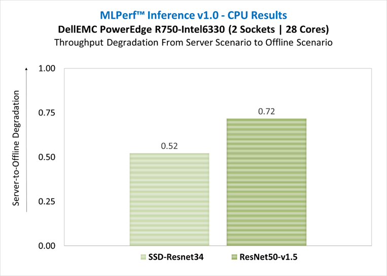
Figure 3: Throughput degradation from server scenario to offline scenario
Results submission v0.7 versus v1.0
In this section we compare the results from submission v0.7 versus this submission v1.0 to determine how the performance improved from servers with 2nd gen Xeon scalable processors vs. 3rd gen. The table below shows the server specifications used on each submission:
| Dell EMC Server for Submission v0.7 | Dell EMC Server for Submission v1.0 |
System Name | PowerEdge R740xd | PowerEdge R750 |
Host Processor Model Name | Intel(R) Xeon(R) Platinum 8280M | Intel(R) Xeon(R) Gold 6330 |
Host Processor Generation | 2nd | 3rd |
Host Processors per Node | 2 | 2 |
Host Processor Core Count | 28 | 28 |
Host Processor Frequency | 2.70 GHz | 2.00 GHz |
Host Processor TDP | 205W | 205W |
Host Memory Capacity | 376GB - 2 DPC 3200 MHz | 1TB - 1 DPC 3200 MHz |
Host Storage Capacity | 1.59TB | 1.5TB |
Host Storage Type | SATA | NVMe |
ResNet50-v1.5 in Offline Scenario | Submission v0.7 vs. v1.0
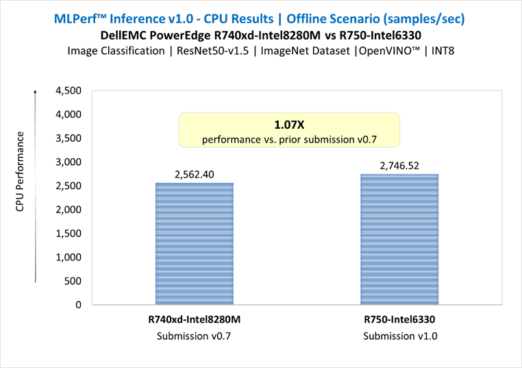
Figure 4: ResNet50-v1.5 in Offline Scenario | Submission v0.7 vs. v1.0
ResNet50-v1.5 in Server Scenario | Submission v0.7 vs. v1.0
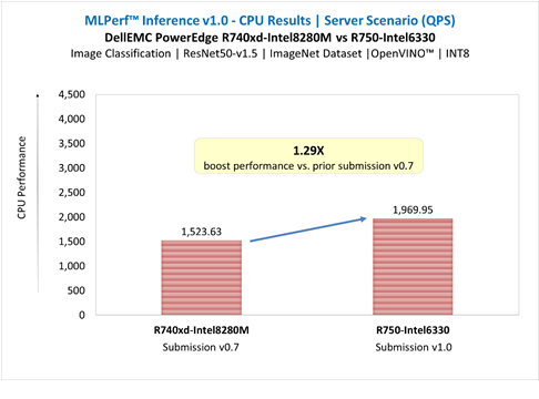
Figure 5: ResNet50-v1.5 in Server Scenario | Submission v0.7 vs. v1.0
SSD-ResNet34 in Offline Scenario | Submission v0.7 vs. v1.0
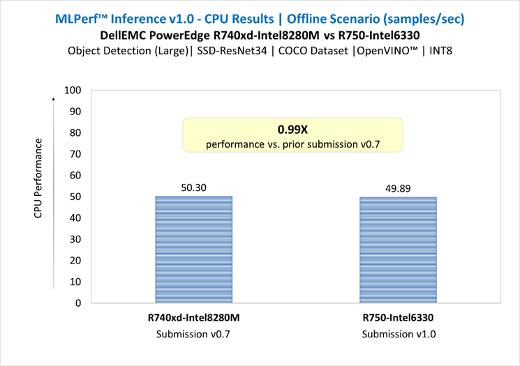
Figure 6: SSD-ResNet34 in Offline Scenario | Submission v0.7 vs. v1.0
SSD-ResNet34 in Server Scenario | Submission v0.7 vs. v1.0
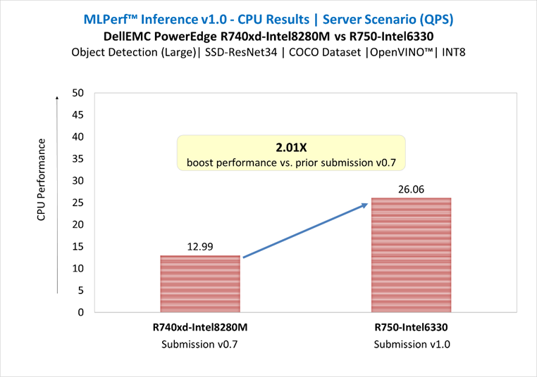
Figure 7: SSD-ResNet34 in Server Scenario | Submission v0.7 vs. v1.0
Conclusion
Both the Gold 6330 and the previous generation Platinum 8280 were chosen for this test because they have 28 cores and a memory interface that operates at 2933Mt/s. Customers with more demanding requirements could also consider higher performing variants of the 3rd Gen Intel® Xeon® scalable processor family up to the 40 core Platinum 8380 which uses a memory interface capable of 3200MT/s.
- The two-socket (dual CPU) server Dell EMC PowerEdge R750 equipped with 3rd Gen Intel® Xeon® scalable processors delivered:
- Up to 1.29X boost performance for image classification and up to 2.01X boost performance for object detection large in server scenario, compared to prior submission of PowerEdge R740xd equipped with 2nd Gen Intel® Xeon® processors.
- For ResNet50-v1.5 benchmark, there was a loss degradation around 28% from server scenario (constrained latency) to offline scenario (unconstrained latency). For SSD-ResNet34 benchmark, the loss was around 48%. These results demonstrate the complexity of server scenario in terms of latency constraints and input queries generation. The throughput degradation from server scenario is an indication of how well the system handles the latency constraint requirements, and it could be related to several factors such as the hardware architecture, the batching management, the inference software stack used to run the benchmarks. It is recommended to conduct performance analysis of the system including both scenarios.
- PowerEdge R750 server drives enhanced performance to suite computer vision inferencing tasks, as well as other complex workloads such as database and advanced analytics, VDI, AI, DL, and ML in datacenters deployments; it is an ideal solution for data center modernization to drive operational efficiency, lead higher productivity, and maximize total cost of ownership (TCO).
Citation
@misc{reddi2019mlperf,
title={MLPerf™ Inference Benchmark},
author={Vijay Janapa Reddi and Christine Cheng and David Kanter and Peter Mattson and Guenther Schmuelling and Carole-Jean Wu and Brian Anderson and Maximilien Breughe and Mark Charlebois and William Chou and Ramesh Chukka and Cody Coleman and Sam Davis and Pan Deng and Greg Diamos and Jared Duke and Dave Fick and J. Scott Gardner and Itay Hubara and Sachin Idgunji and Thomas B. Jablin and Jeff Jiao and Tom St. John and Pankaj Kanwar and David Lee and Jeffery Liao and Anton Lokhmotov and Francisco Massa and Peng Meng and Paulius Micikevicius and Colin Osborne and Gennady Pekhimenko and Arun Tejusve Raghunath Rajan and Dilip Sequeira and Ashish Sirasao and Fei Sun and Hanlin Tang and Michael Thomson and Frank Wei and Ephrem Wu and Lingjie Xu and Koichi Yamada and Bing Yu and George Yuan and Aaron Zhong and Peizhao Zhang and Yuchen Zhou}, year={2019},
eprint={1911.02549}, archivePrefix={arXiv}, primaryClass={cs.LG}