Llama 2: Efficient Fine-tuning Using Low-Rank Adaptation (LoRA) on Single GPU
Wed, 24 Apr 2024 14:23:28 -0000
|Read Time: 0 minutes
Introduction
With the growth in the parameter size and performance of large-language models (LLM), many users are increasingly interested in adapting them to their own use case with their own private dataset. These users can either search the market for an Enterprise-level application which is trained on large corpus of public datasets and might not be applicable to their internal use case or look into using the open-source pre-trained models and then fine-tuning them on their own proprietary data. Ensuring efficient resource utilization and cost-effectiveness are crucial when choosing a strategy for fine-tuning a large-language model, and the latter approach offers a more cost-effective and scalable solution given that it’s trained with known data and able to control the outcome of the model.
This blog investigates how Low-Rank Adaptation (LoRA) – a parameter effective fine-tuning technique – can be used to fine-tune Llama 2 7B model on single GPU. We were able to successfully fine-tune the Llama 2 7B model on a single Nvidia’s A100 40GB GPU and will provide a deep dive on how to configure the software environment to run the fine-tuning flow on Dell PowerEdge R760xa featuring NVIDIA A100 GPUs.
This work is in continuation to our previous work, where we performed an inferencing experiment on Llama2 7B and shared results on GPU performance during the process.
Memory bottleneck
When finetuning any LLM, it is important to understand the infrastructure needed to load and fine-tune the model. When we consider standard fine-tuning, where all the parameters are considered, it requires significant computational power to manage optimizer states and gradient checkpointing. The optimizer states and gradients usually result in a memory footprint which is approximately five times larger than the model itself. If we consider loading the model in fp16 (2 bytes per parameter), we will need around 84 GB of GPU memory, as shown in figure 1, which is not possible on a single A100-40 GB card. Hence, to overcome this memory capacity limitation on a single A100 GPU, we can use a parameter-efficient fine-tuning (PEFT) technique. We will be using one such technique known as Low-Rank Adaptation (LoRA) for this experiment.
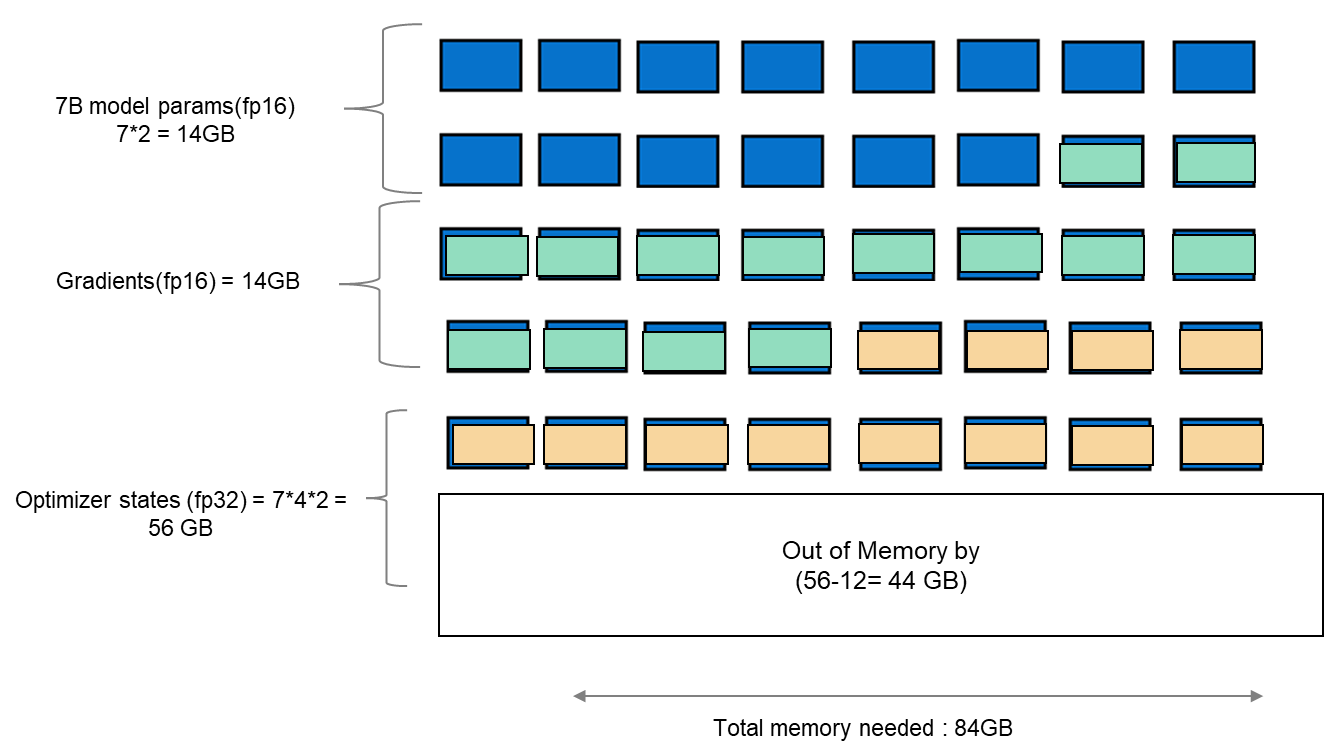
Figure 1. Schematic showing memory footprint of standard fine-tuning with Llama 27B model.
Fine-tuning method
LoRA is an efficient fine-tuning method where instead of finetuning all the weights that constitute the weight matrix of the pre-trained LLM, it optimizes rank decomposition matrices of the dense layers to change during adaptation. These matrices constitute the LoRA adapter. This fine-tuned adapter is then merged with the pre-trained model and used for inferencing. The number of parameters is determined by the rank and shape of the original weights. In practice, trainable parameters vary as low as 0.1% to 1% of all the parameters. As the number of parameters needing fine-tuning decreases, the size of gradients and optimizer states attached to them decrease accordingly. Thus, the overall size of the loaded model reduces. For example, the Llama 2 7B model parameters could be loaded in int8 (1 byte), with 1 GB trainable parameters loaded in fp16 (2 bytes). Hence, the size of the gradient (fp16), optimizer states (fp32), and activations (fp32) aggregates to approximately 7-9 GB. This brings the total size of the loaded model to be fine-tuned to 15-17 GB, as illustrated in figure 2.
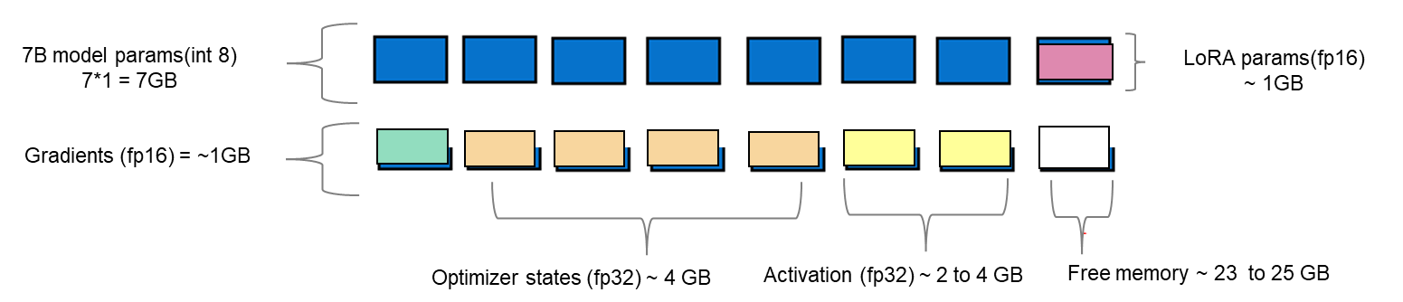
Figure 2. Schematic showing an example of memory footprint of LoRA fine tuning with Llama 2 7B model.
Experimental setup
A model characterization gives readers valuable insight into GPU memory utilization, training loss, and computational efficiency measured during fine-tuning by varying the batch size and observing out-of-memory (OOM) occurrence for a given dataset. In table 1, we show resource profiling when fine-tuning Llama 2 7B-chat model using LoRA technique on PowerEdge R760xa with 1*A100-40 GB on Open- source SAMsum dataset. To measure tera floating-point operations (TFLOPs) on the GPU, the DeepSpeed Flops Profiler was used. Table 1 gives the detail on the system used for this experiment.
Table 1. Actual memory footprint of Llama 27B model using LoRA technique in our experiment.
Trainable params (LoRA) | 0.0042 B (0.06% of 7B model) |
7B model params(int8) | 7 GB |
Lora adapter (fp16) | 0.0084 GB |
Gradients (fp32) | 0.0168 GB |
Optimizer States(fp32) | 0.0168 GB |
Activation | 2.96 GB |
Total memory for batch size 1 | 10 GB = 9.31 GiB |
System configuration
In this section, we list the hardware and software system configuration of the R760xa PowerEdge server used in this experiment for the fine-tuning work of Llama-2 7B model.
Figure 3. R760XA Specs
Table 2. Hardware and software configuration of the system
Component | Details |
Hardware | |
Compute server for inferencing | PowerEdge R760xa |
GPUs | Nvidia A100-40GB PCIe CEM GPU |
Host Processor Model Name | Intel(R) Xeon(R) Gold 6454S (Sapphire Rapids) |
Host Processors per Node | 2 |
Host Processor Core Count | 32 |
Host Processor Frequency | 2.2 GHz |
Host Memory Capacity | 512 GB, 16 x 32GB 4800 MT/s DIMMs |
Host Storage Type | SSD |
Host Storage Capacity | 900 GB |
Software | |
Operating system | Ubuntu 22.04.1 |
Profiler | |
Framework | PyTorch |
Package Management | Anaconda |
Dataset
The SAMsum dataset – size 2.94 MB – consists of approximately 16,000 rows (Train, Test, and Validation) of English dialogues and their summary. This data was used to fine-tune the Llama 2 7B model. We preprocess this data in the format of a prompt to be fed to the model for fine-tuning. In the JSON format, prompts and responses were used to train the model. During this process, PyTorch batches the data (about 10 to 11 rows per batch) and concatenates them. Thus, a total of 1,555 batches are created by preprocessing the training split of the dataset. These batches are then passed to the model in chunks for fine-tuning.
Fine-tuning steps
- Download the Llama 2 model
- The model is available either from Meta’s git repository or Hugging Face, however to access the model, you will need to submit the required registration form for Meta AI license agreement
- The details can be found in our previous work here
- Convert the model from the Meta’s git repo to a Hugging face model type in order to use the PEFT libraries used in the LoRA technique
- Use the following commands to convert the model
## Install HuggingFace Transformers from source pip freeze | grep transformers ## verify it is version 4.31.0 or higher
git clone git@github.com:huggingface/transformers.git
cd transformers
pip install protobuf
python src/transformers/models/llama/convert_llama_weights_to_hf.py \
--input_dir /path/to/downloaded/llama/weights --model_size 7B --output_dir /output/path
- Use the following commands to convert the model
- Build a conda environment and then git clone the example fine-tuning recipes from Meta’s git repository to get started
- We have modified the code base to include Deepspeed flops profiler and nvitop to profile the GPU
- Load the dataset using the dataloader library of hugging face and, if need be, perform preprocessing
- Input the config file entries with respect to PEFT methods, model name, output directory, save model location, etc
- The following is the example code snippet
train_config: model_name: str="path_of_base_hugging_face_llama_model" run_validation: bool=True batch_size_training: int=7 num_epochs: int=1 val_batch_size: int=1 dataset = "dataset_name" peft_method: str = "lora" output_dir: str = "path_to_save_fine_tuning_model" save_model: bool = True |
6. Run the following command to perform fine tuning on a single GPU
python3 llama_finetuning.py --use_peft --peft_method lora --quantization --model_name location_of_hugging_face_model |
Figure 4 shows fine tuning with LoRA technique on 1*A100 (40GiB) with Batch size = 7 on SAMsum dataset, which took 83 mins to complete.
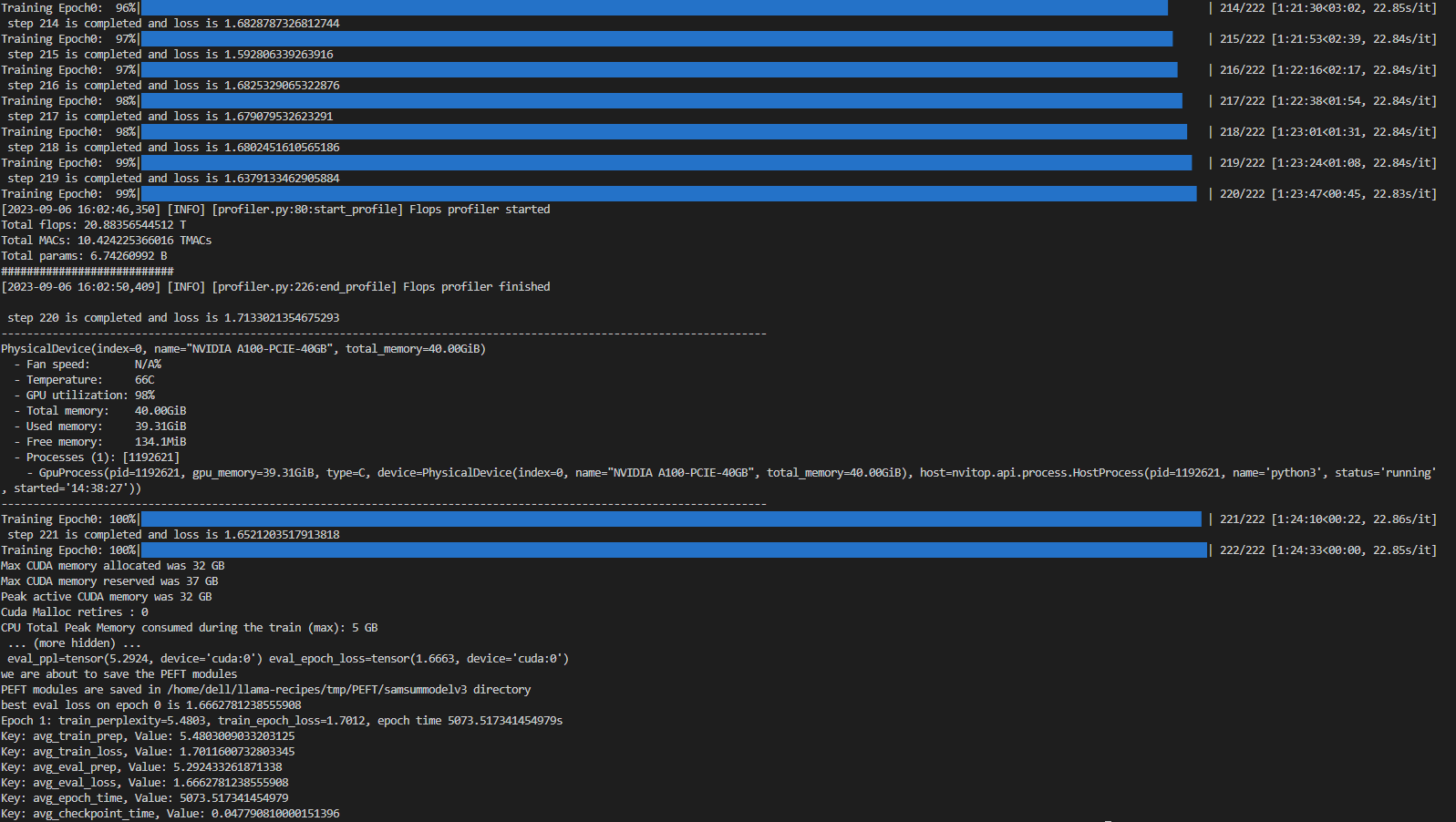
Figure 4. Example screenshot of fine-tuning with LoRA on SAMsum dataset
Experiment results
The fine-tuning experiments were run at batch sizes 4 and 7. For these two scenarios, we calculated training losses, GPU utilization, and GPU throughput. We found that at batch size 8, we encountered an out-of-memory (OOM) error for the given dataset on 1*A100 with 40 GB.
When a dialogue was sent to the base 7B model, the summarization results are not proper as shown in figure 5. After fine-tuning the base model on the SAMsum dataset, the same dialogue prompts a proper summarized result as shown in figure 6. The difference in results shows that fine-tuning succeeded.
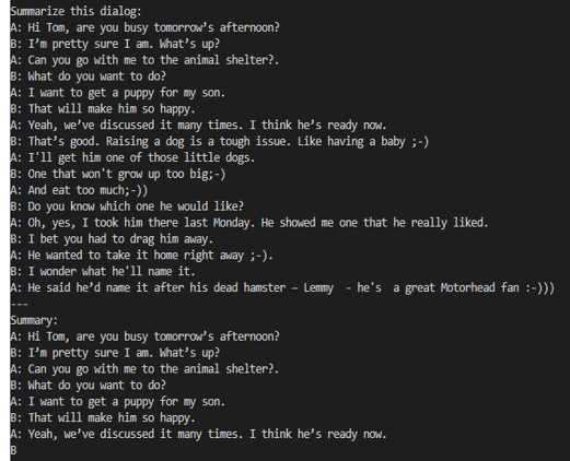
Figure 5. Summarization results from the base model.
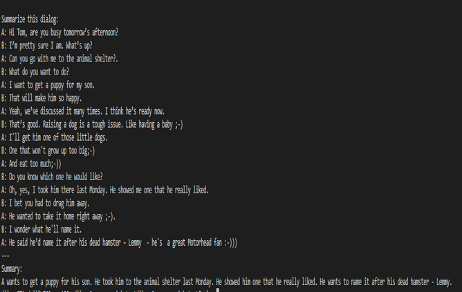
Figure 6. Summarization results from the fine-tuned model.
Figures 7 and 8 show the training losses at batch size 4 and 7 respectively. We found that even after increasing the batch size by approximately 2x times, the model training performance did not degrade.
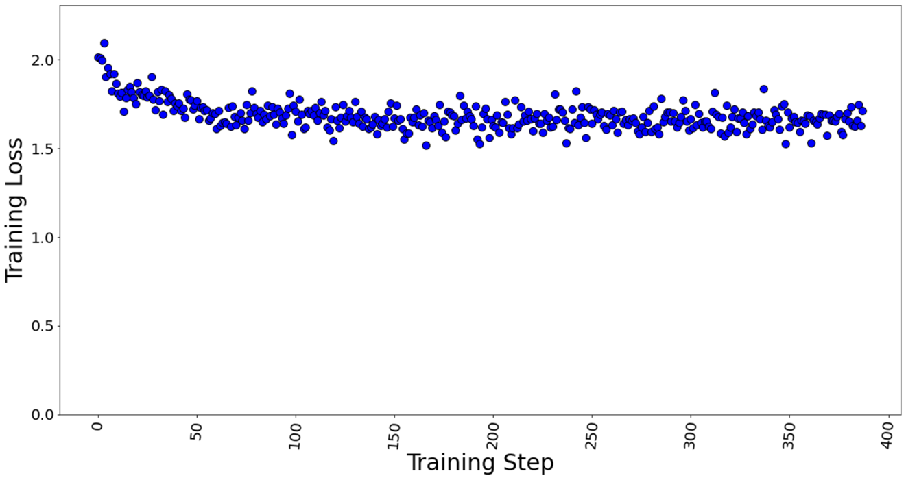
Figure 7. Training loss with batch size = 4, a total of 388 training steps in 1 epoch.
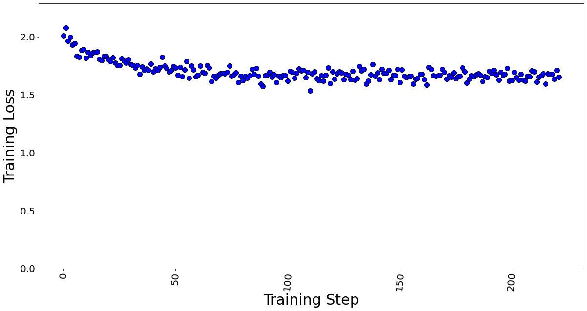
Figure 8. Training loss with batch size = 7, a total of 222 training steps in 1 epoch.
The GPU memory utilization was captured with LoRA technique in Table 3. At batch size 1, used memory was 9.31 GB. At batch size of 4, used memory was 26.21 GB. At batch size 7, memory used was 39.31 GB. Going further, we see an OOM at batch size 8 for 40 GB GPU card. The memory usage remains constant throughout fine-tuning, as shown in Figure 9, and is dependent on the batch size. We calculated the reserved memory per batch to be 4.302 GB on 1*A100.
Table 3. The GPU memory utilization is captured by varying the max. batch size parameter.
Max. Batch Size | Steps in 1 Epoch | Total Memory (GiB) | Used Memory (GiB) | Free Memory (GiB) |
1 | 1,555 | 40.00 | 9.31 | 30.69 |
4 | 388 | 40.00 | 26.21 | 13.79 |
7 | 222 | 40.00 | 39.31 | 0.69 |
8 | Out of Memory Error |
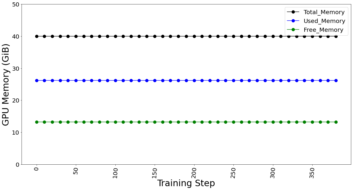
Figure 9. GPU memory utilization for batch size 4 (which remains constant for fine-tuning)
The GPU TFLOP was determined using DeepSpeed Profiler, and we found that FLOPs vary linearly with the number of batches sent in each step, indicating that FLOPs per token is the constant.
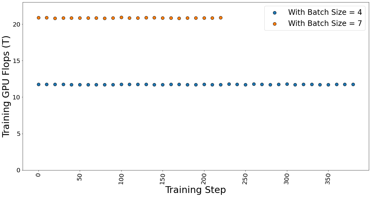
Figure 10. Training GPU TFlops for batch sizes 4 and 7 while fine-tuning the model.
The GPU multiple-accumulate operations (MACs), which are common operations performed in deep learning models, are also determined. We found that MACs also follow a linear dependency on the batch size and hence constant per token.
Figure 11. GPU MACs for batch sizes 4 and 7 while the fine-tuning the model.
The time taken for fine-tuning, which is also known as epoch time, is given in table 4. It shows that the training time does not vary much, which strengthens our argument that the FLOPs per token is constant. Hence, the total training time is independent of the batch size.
Table 4. Data showing the time taken by the fine-tuning process.
Max. Batch Size | Steps in 1 Epoch | Epoch time (secs) |
4 | 388 | 5,003 |
7 | 222 | 5,073 |
Conclusion and Recommendation
- We show that using a PEFT technique like LoRA can help reduce the memory requirement for fine-tuning a large-language model on a proprietary dataset. In our case, we use a Dell PowerEdge R760xa featuring the NVIDIA A100-40GB GPU to fine-tune a Llama 2 7B model.
- We recommend using a lower batch size to minimize automatic memory allocation, which could be utilized in the case of a larger dataset. We have shown that a lower batch size affects neither the training time nor training performance.
- The memory capacity required to fine-tune the Llama 2 7B model was reduced from 84GB to a level that easily fits on the 1*A100 40 GB card by using the LoRA technique.
Resources
- Llama 2: Inferencing on a Single GPU
- LoRA: Low-Rank Adaptation of Large Language Models
- Hugging Face Samsum Dataset
Author: Khushboo Rathi khushboo_rathi@dell.com | www.linkedin.com/in/khushboorathi
Co-author: Bhavesh Patel bhavesh_a_patel@dell.com | www.linkedin.com/in/BPat
Related Blog Posts
Running Meta Llama 3 Models on Dell PowerEdge XE9680
Thu, 02 May 2024 17:54:12 -0000
|Read Time: 0 minutes
Introduction
Recently, Meta has open-sourced its Meta Llama 3 text-to-text models with 8B and 70B sizes, which are the highest scoring LLMs that have been open-sourced so far in their size ranges, in terms of quality of responses[1]. In this blog, we will run those models on the Dell PowerEdge XE9680 server to show their performance and improvement by comparing them to the Llama 2 models.
Open-sourcing the Large Language Models (LLMs) enables easy access to this state-of-the-art technology and has accelerated innovations in the field and adoption for different applications. As shown in Table 1, this round of Llama 3 release includes the following five models in total, including two pre-trained models with sizes of 8B and 70B and their instruction-tuned versions, plus a safeguard version for the 8B model[2].
Table 1: Released Llama 3 Models
Model size (Parameters) | Model names | Context | Training tokens | Vocabulary length |
8B |
| 8K |
15T |
128K |
70B |
|
Llama 3 is trained on 15T tokens which is 7.5X the number of tokens on which Llama 2 was trained. Training with large, high-quality datasets and refined post-training processes improved Llama 3 model’s capabilities, such as reasoning, code generation, and instruction following. Evaluated across main accuracy benchmarks, the Llama 3 model not only exceeds its precedent, but also leads over other main open-source models by significant margins. The Llama 3 70B instruct model shows close or even better results compared to the commercial closed-source models such as Gemini Pro[1].
The model architecture of Llama 3 8B is similar to that of Llama 2 7B with one significant difference. Besides a larger parameter size, the Llama 3 8B model uses the group query attention (GQA) mechanism instead of the multi-head attention (MHA) mechanism used in the Llama 2 7B model. Unlike MHA which has the same number of Q (query), K (key), and V (value) matrixes, GQA reduces the number of K and V matrixes required by sharing the same KV matrixes across grouped Q matrixes. This reduces the memory required and improves computing efficiency during the inferencing process[3]. In addition, the Llama 3 models improved the max context window length to 8192 compared to 4096 for the Llama 2 models. Llama 3 uses a new tokenizer called tik token that expands the vocabulary size to 128K when compared to 32K used in Llama 2. The new tokenization scheme offers improved token efficiency, yielding up to 15% fewer tokens compared to Llama 2 based on Meta’s benchmark[1].
This blog focuses on the inference performance tests of the Llama 3 models running on the Dell PowerEdge XE9680 server, especially, the comparison with Llama 2 models, to show the improvements in the new generation of models.
Test setup
The server we used to benchmark the performance is the PowerEdge XE9680 with 8x H100 GPUs[4]. The detailed server configurations are shown in Table 2.
Table 2: XE9680 server configuration
System Name | PowerEdge XE9680 |
Status | Available |
System Type | Data Center |
Number of Nodes | 1 |
Host Processor Model | 4th Generation Intel® Xeon® Scalable Processors |
Host Process Name | Intel® Xeon® Platinum 8470 |
Host Processors per Node | 2 |
Host Processor Core Count | 52 |
Host Processor Frequency | 2.0 GHz, 3.8 GHz Turbo Boost |
Host Memory Capacity and Type | 2TB, 32x 64 GB DIMM, 4800 MT/s DDR5 |
Host Storage Capacity | 1.8 TB, NVME |
GPU Number and Name | 8x H100 |
GPU Memory Capacity and Type | 80GB, HBM3 |
GPU High-speed Interface | PCIe Gen5 / NVLink Gen4 |
The XE9680 is the ideal server, optimized for AI workloads with its 8x NVSwitch interconnected H100 GPUs. The high-speed NVLink interconnect allows deployment of large models like Llama 3 70B that need to span multiple GPUs for best performance and memory capacity requirements. With its 10 PCIe slots, the XE9680 also provides a flexible PCIe architecture that enables a variety of AI fabric options.
For these tests, we deployed the Llama 3 models Meta-Llama-3-8B and Meta-Llama-3-70B, and the Llama 2 models Llama-2-7b-hf and Llama-2-70b-hf. These models are available for download from Hugging Face after permission approved by Meta. For a fair comparison between Llama 2 and Llama 3 models, we ran the models with native precision (float16 for Llama 2 models and bfloat16 for Llama 3 models) instead of any quantized precision.
Given that it has the same basic model architecture as Llama 2, Llama 3 can easily be integrated into any available software eco-system that currently supports the Llama 2 model. For the experiments in this blog, we chose NVIDIA TensorRT-LLM latest release (version 0.9.0) as the inference framework. NVIDIA CUDA version was 12.4; the driver version was 550.54.15. The operating system for the experiments was Rocky Linux 9.1.
Knowing that the Llama 3 improved accuracy significantly, we first concentrated on the inferencing speed tests. More specifically, we tested the Time-to-First-Token (TTFT) and throughput over different batch sizes for both Llama 2 and Llama 3 models, as shown in the Results section. To make the comparison between two generations of models easy, and to mimic a summarization task, we kept the input token length and output token length at 2048 and 128 respectively for most of the experiments. We also measured throughput of the Llama 3 with the long input token length (8192), as one of the most significant improvements. Because H100 GPUs support the fp8 data format for the models with negligible accuracy loss, we measured the throughput under long input token length for the Llama 3 model at fp8 precision.
Results
Figure 1. Inference speed comparison: Llama-3-70b vs Llama-2-70b: Time-to-First-Token
Figure 2: Inference speed comparison: Llama-3-70b vs Llama-2-70b: Throughput
Figures 1 and 2 show the inference speed comparison with the 70b Llama 2 (Llama-2-70b) and Llama 3 (Llama-3-70b) models running across eight H100 GPUs in a tensor parallel (TP=8) fashion on an XE9680 server. From the test results, we can see that for both TTFT (Figure 1) and throughput (Figure 2), the Llama 3 70B model has a similar inference speed to the Llama 2 70b model. This is expected given the same size and architecture of the two models. So, by deploying Llama 3 instead of Llama 2 on an XE9680, organizations can immediately see a big boost in accuracy and quality of responses, using the same software infrastructure, without any impact to latency or throughput of the responses.
Figure 3. Inference speed comparison: Llama-3-8b vs Llama-2-7b: Time-to-First-Token
Figure 4: Inference speed comparison: Llama-3-8b vs Llama-2-7b: Throughput
Figures 3 and 4 show the inference speed comparison with the 7b Llama 2 (Llama-2-7b) and 8b Llama 3 (Llama-3-8b) models running on a single H100 GPU on an XE9680 server. From the results, we can see the benefits of using the group query attention (GQA) in the Llama 3 8B architecture, in terms of reducing the GPU memory footprint in the prefill stage and speeding up the calculation in the decoding stage of the LLM inferencing. Figure 3 shows that Llama 3 8B has a similar response time in generating the first token even though it is a 15% larger model compared to Llama-2-7b. Figure 4 shows that Llama-3-8b has higher throughput than Llama-2-7b when the batch size is 4 or larger. The benefits of GQA grow as the batch size increases. We can see from the experiments that:
- the Llama-2-7b cannot run at a batch size of 64 or larger with the 16-bit precision and given input/output token length, because of the OOM (out of memory) error
- the Llama-3-8b can run at a batch size of 128, which gives more than 2x throughput with the same hardware configuration
Figure 5: Llama-3-70b throughput under 8192 input token length
Another improvement of the Llama 3 model: it supports a max input token length of 8192, which is 2x of that of a Llama 2 model. We tested it with the Llama-3-70b model running on 8 H100 GPUs of the XE9680 server. The results are shown in Figure 5. The throughput is linearly proportional to the batch size tested and can achieve 271 tokens/s at a batch size of 16, indicating that more aggressive quantization techniques can further improve the throughput.
Conclusion
In this blog, we investigated the Llama 3 models that were released recently, by comparing their inferencing speed with that of the Llama 2 models by running on a Dell PowerEdge XE9680 server. With the numbers collected through experiments, we showed that not only is the Llama 3 model series a big leap in terms of the quality of responses, it also has great inferencing advantages in terms of high throughput with a large achievable batch size, and long input token length. This makes Llama 3 models great candidates for those long context and offline processing applications.
Authors: Tao Zhang, Khushboo Rathi, and Onur Celebioglu
[1] Meta AI, “Introducing Meta Llama 3: The most capable openly available LLM to date”, https://ai.meta.com/blog/meta-llama-3/.
[3] J. Ainslie et. al, “GQA: Training Generalized Multi-Query Transformer Models from Multi-Head Checkpoints”, https://arxiv.org/abs/2305.13245
Scaling Hardware and Computation for Practical Deep Learning Applications in Healthcare
Fri, 01 Dec 2023 15:26:29 -0000
|Read Time: 0 minutes
Medical practice requires analysis of large volumes of data spanning multiple modalities. While these can be as simple as numeric lab results, at the other extreme are high-complexity data such as magnetic resonance imaging or decades-worth of text-based clinical documentation which may be present in medical records. Oftentimes, small details buried within piles of clinical information are critical to obtaining a complete clinical picture. Many deep learning methods developed in recent years have focused on very short “sequence lengths” – the term used to describe the number of words or pixels that a model can ingest – of images and text compared to those encountered in clinical practice. How do we scale such tools to model this breadth of clinical data appropriately and efficiently?
In the following blog, we discuss ways to tackle the compute requirements of developing transformer-based deep learning tools for healthcare data from the hardware, data processing, and modeling perspectives. To do so, we present a practical application of Flash Attention using a series of experiments performing an analysis of the publicly available Kaggle RSNA Screening Mammography Breast Cancer Detection challenge, which contains 54,706 images of 11,913 patients. Breast cancer affects 1 in 8 women and is the second leading cause of cancer death. As such, screening mammography is one of the most performed imaging-based medical screening procedures, which offers a clinically relevant and data-centric case study to consider.
Data Primer
To detect breast cancer early when treatments are most effective, high-resolution x-ray images are taken of breast tissue to identify areas of abnormality which require further examination by biopsy or more detailed imaging. Typically, two views are acquired:
- Craniocaudal (CC) – taken from the head-to-toe perspective
- Mediolateral oblique (MLO) – taken at an angle
The dataset contains DICOM-formatted images which must be pre-processed in a standard fashion prior to model training. We detail the data preparation pipeline in figure 1. The CC and MLO views of each study are identified, flipped horizontally if necessary, cropped, and combined to form the model input image. We wrap the standard PyTorch Dataset class to load images and preprocess them for training.
A more in-depth look at the system for data pre-processing is as follows:
- For each breast with a corresponding cancer label, the CC and MLO views are extracted, and the image data are normalized. Right-sided images are horizontally flipped so that the tissue is to the left side of the image, as shown.
- Images are cropped to the region of interest (ROI), excluding areas of black or non-tissue artifacts.
- Images are resized, maintaining aspect ratio, and tiled to a square of the output size of interest, with the CC view occupying the left half of the output and the MLO view occupying the right.
An important consideration is whether to perform this processing within the dataloader while training or to save a pre-processed version of the dataset. The former approach allows for iteration on different processing strategies without modifying the dataset itself, providing greater ease of experimentation. However, this level of processing during training may limit the rate at which data can be fed to the graphics processing unit (GPU) for training, resulting in time and monetary inefficiencies. In contrast, the latter approach requires that multiple versions of the dataset be saved locally, which is potentially prohibitive when working with large dataset sizes and storage space and/or network limitations. For the purpose of this blog post, to benchmark GPU hardware and training optimizations, we use the second method, saving data on local solid state drives connected via NVMe to ensure GPU saturation despite processor differences. In general, before implementing the training optimizations described below, it is important to first ensure that dataloading does not bottleneck the overall training process.
Scaling Up
Naturally, increasing the capability and amount of compute available for model training yields direct benefits. To demonstrate the influence of hardware on run time, we present a simple 20-epoch training experiment using the same dataset on three different servers, shown in figure 2:
- Dell XE8545 with 4x NVIDIA A100-SXM4 40GB GPUs and an AMD EPYC 7763 with 64 cores
- Dell R750xa with 4x NVIDIA A100 80GB GPUs and an Intel Xeon Gold 5320 processor with 26 cores
- Dell XE9680 server with 8 NVIDIA HGX A100 80GB SXM4 GPUs and an Intel Xeon Platinum 8470 processor with 52 cores
Input data into the model shown in figure 2 were 512x512 with a patch size of 16. Batch size was 24 per GPU on the 40GB and 64 on the 80GB servers.
Parameters remain the same for each run, except that batch size has been increased to maximally utilize GPU memory on the R750xa and XE9680 compared with the XE8545. Gradient accumulation is performed to maintain a constant global batch size per model weight update for each run. We see a clear improvement in runtime as the hardware is scaled up, demonstrating how increased compute capability directly yields time savings which enables researchers to efficiently iterate on experiments and train effective models.
In conjunction with hardware, sequence lengths of data should be carefully considered given the application of interest. The selected tokenization scheme directly impacts sequence length of input data, such as the patch size selected as input to a vision transformer. For example, a patch size of 16 on a 1024x1024 image will result in a sequence length of 4,096 (Height*Width/Patch Size2) while a patch size of 8 will result in a sequence length of 16,384. While GPUs increasingly feature more memory, they present an upper bound on the sequence length that can practicably be considered. Smaller patch sizes – and thus, longer sequences – will result in slower throughput via smaller batch sizes and a greater number of computations, as shown in figure 3. However, larger images sizes coupled with smaller patch sizes are particularly relevant in analysis of mammography and other applications in which fine-resolution features are of interest.
The data illustrated in figure 3 are taken from a run of twenty epochs using an image size of 512x512 and tested on an 8xA100 (80 GB) server.
Flash Attention – Experiments
Recently, Dao et al. have published on Flash Attention (https://arxiv.org/abs/2205.14135), a technique aimed at more efficiently accomplishing the computations involved within transformers via minimizing GPU high-bandwidth memory and the on-chip SRAM. Their reported findings are impressive, yielding 2-3x speedups during an attention forward and backwards pass while also having 3-20x smaller memory requirements.
Using a Dell XE9680 server with 8 NVIDIA HGX A100 80GB SXM4 GPUs and an Intel Xeon Platinum 8470 processor with 52 cores, we provide a practical demonstration of potential applications for Flash Attention and vision transformers in healthcare. Specifically, we performed experiments to demonstrate how sequence length (determined by patch size and image size) and Flash Attention impact training time. To limit confounding variables, all images were pre-sized on disk and directly loaded into the vision transformer without any permutations. For the vision transformer, the ViT-Base from Huggingface was used. For Flash Attention, the Encoder from the x_transformers library was used, shown being implemented in the following code.
All tests were carried out with the Huggingface trainer using an effective batch size of 128 per GPU, “brain" floating-point 16 data, and across twenty epochs at patch sizes of 8, 16, and 32 with image sizes of 384, 512, 1024, and 2048.
from x_transformers import ViTransformerWrapper, Encoder class FlashViT(nn.Module): def __init__(self, encoder = ViTransformerWrapper( image_size = args.img_size, patch_size = args.patch_size, num_classes = 2, channels=3, attn_layers = Encoder( dim = 768, depth = 12, heads = 12, attn_flash=True ) ), super().__init__() self.encoder = encoder def forward(self, pixel_values:torch.tensor, labels:torch.tensor): """ pixel_values: [batch,channel,ht,wt] of pixel values labels: labels for each image """ logits = self.encoder(pixel_values) return {'loss':F.cross_entropy(logits,labels),'logits':logits} model = FlashViT()
Figure 4 demonstrates the pronounced benefit of using Flash Attention within a vision transformer with respect to model throughput. With the exception of the two smallest image sizes and largest patch size (and thus shortest sequence length), Flash Attention resulted in a marked speed increase across all other perturbations. The speed-up range across patch sizes was:
- Patch size of 8: 3.0 - 4.2x
- Patch size of 16: 2.8 – 4.0x
- Patch size of 32: 0 - 2.3x
Another benefit demonstrated in these experiments is the additional image and patch size combinations achievable only with Flash Attention due to the reduced GPU memory requirement. Non-Flash Attention models could only be used on image sizes of 2,048 if a patch size of 32 was used (sequence length of 4,096), whereas Flash Attention was capable of running on patch sizes of 8 and 16. Even at shorter sequence lengths (576 - 384x384 image, patch size of 16), there was 2.3x less memory used for Flash Attention. Use of Flash Attention will also be critical when considering larger transformer models, with ViT-Huge having more than 7x the parameters than ViT-Base. In conjunction with hardware-enabling distributed training at scale such as the Dell XE9680, these optimizations will enable new findings at unprecedented scales.
Takeaways
We have described methods by which the benefits of transformer-based models can be scaled to the longer sequences which medical data often require. Notably, we demonstrate the benefits of implementing Flash Attention to a vision encoder. Flash Attention presents marked benefit from a modeling perspective, from shorter runtimes (and thus lower cost) to better image encoding (longer sequence lengths). Moreover, we show that these benefits scale substantially along with sequence length, making them indispensable for practitioners aiming to model the full complexity of hospital data. As machine learning continues to grow in healthcare, tight collaborations between hospitals and technology manufactures are thus essential to allow for greater compute resources to input higher-quality data into machine learning models.
Resources
- Dell XE9680 Technical Guide: https://www.delltechnologies.com/asset/en-ca/products/servers/technical-support/poweredge-xe9680-technical-guide.pdf
- Dell R750xa Technical Guide: https://i.dell.com/sites/csdocuments/Product_Docs/en/poweredge-r750xa-technical-guide.pdf
- Dell XE8545 Technical Guide: https://i.dell.com/sites/csdocuments/product_docs/en/poweredge-xe8545-technical-guide.pdf
Authors:
Jonathan Huang, MD/PhD Candidate, Research & Development, Northwestern Medicine
Matthew Wittbrodt, Solutions Architect, Research & Development, Northwestern Medicine
Alex Heller, Director, Research & Development, Northwestern Medicine
Mozziyar Etemadi, Clinical Director, Advanced Technologies, Northwestern Medicine
Bhavesh Patel, Sr. Distinguished Engineer, Dell Technologies
Bala Chandrasekaran, Technical Staff, Dell Technologies
Frank Han, Senior Principal Engineer, Dell Technologies