Beyond Open-Source LLMs: Tailoring Models for Your Needs

The open-source LLM landscape is booming! But with so many options, choosing the right model can be overwhelming. What if you need a model with both domain-specific knowledge and diverse generation capabilities? Enter model merging, a powerful technique to unlock the full potential of LLMs.

Model merging: Unlocking model versatility

Model merging allows you to combine the strengths of different pre-trained models without additional training. This creates a "multitask" model, excelling in both specific domains and diverse generation tasks and addressing key challenges in AI like:

• Catastrophic Forgetting: This occurs when a model learning new tasks forgets those previously learned. Merging preserves the original model’s capabilities.
• Multitask Learning: Effectively training a model for multiple tasks can be difficult. Merging offers a way to combine pre-trained models with different strengths.

This blog explores the use of the MergeKit Python library to merge pre-trained LLMs like Mistral-7B-v0.1 and Zephyr-7B-alpha. We'll demonstrate how to create a new model that leverages the strengths of both.

Architecture

There are a variety of methods that can be used during model merging, such as Linear, Spherical Linear Interpolation (SLERP), TIES, DARE, Passthrough, and Task Arithmetic. For the purposes of this blog, we will be using the task arithmetic method, which computes the task vector of each model by subtracting it from the base model weights. This method works best with models that were fine-tuned from common ancestors and have a similar model framework. Hence, in this walk-through, we will merge the fine-tuned version of zephyr-7B with its base model—Mistral-7B—to form our new merged model. Alternatively, you could merge your special domain-specific, highly fine-tuned model of Mistral-7B with the base model of Mistral-7B.

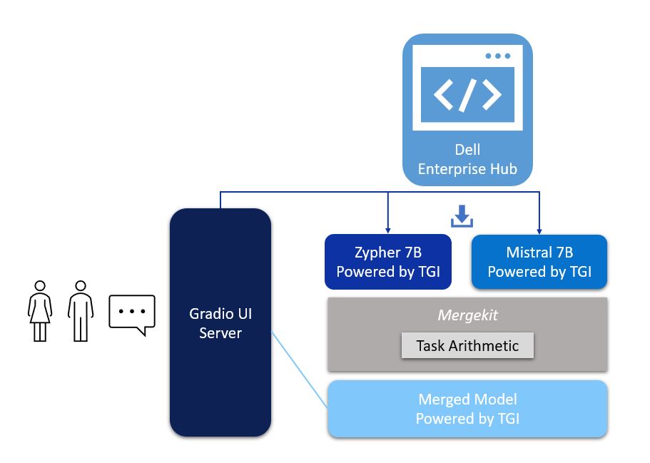
Figure 1. Architecture of model merging deployment, with UI powered by Gradio and Zypher 7B, Mistal 7B and the merged model all powered by TGI from Dell Enterprise Hub

Implementation

The following describes the process for merging two models using mergekit and deploying the merged model to production:

1.  Login with your user access token from Hugging Face.

2. From Dell Enterprise Hub, select the models you would like to merge. For the purposes of this blog, we chose Zephyr-7b-beta and mistralai/Mistral-7B-v0.1

docker run \
    -it \
    --gpus 1 \
    --shm-size 1g \
    -p 80:80 \
    -v /path/on/local_workspace:/Model_zephyr-7b-beta_weights 
    -e NUM_SHARD=1 \
    -e MAX_BATCH_PREFILL_TOKENS=32768 \
    -e MAX_INPUT_TOKENS=8000 \
    -e MAX_TOTAL_TOKENS=8192 \
         registry.dell.huggingface.co/enterprise-dell-inference-huggingfaceh4-zephyr-7b-beta
 
 

docker run \
    --gpus 2 \
    --shm-size 1g \
    -v /path/on/local_workspace:/Model_mistralai-mistral-7b-v0.1  \
    -v /home/$USER/autotrain:/app/autotrain \
         registry.dell.huggingface.co/enterprise-dell-training-mistralai-mistral-7b-v0.1 \
    --model /app/model \
    --project-name fine-tune \
    --data-path /app/data \
    --text-column text \
    --trainer sft \
    --epochs 3 \
    --mixed_precision bf16
    --batch-size 2 \
    --peft \
    --quantization int4
 

3. Once we have the Dell optimized containers, the weights of the models must be stored locally to mount them on our training container. The weights can be found on the /model directory inside the container, as shown here:

#container ID of the image running the model 
 
kradmin@jpnode4:~$ docker ps
CONTAINER ID   IMAGE                                                                                      COMMAND                  CREATED          STATUS          PORTS                                                       NAMES
19c2e634c2ba        registry.dell.huggingface.co/enterprise-dell-inference-huggingfaceh4-zephyr-7b-beta   "/tgi-entrypoint.sh …"   25 seconds ago   Up 25 seconds   0.0.0.0:8888->80/tcp, :::8888->80/tcp                       compassionate_varahamihira
 
#Capture the container ID to execute the docker 
 
kradmin@jpnode4:~$  docker exec -it 19c2e634c2ba bash
 
#copying the weights outside from the container 
root@19c2e634c2ba:/usr/src# cd /model
root@19c2e634c2ba:/model# cp -r /model /Model_zephyr-7b-beta_weights

Now, the weights are stored locally in the folder Model_zephyr-7b-beta_weights outside the container. Follow the same process for the mistral-7b-v0.1 model weights.

4. Retrieve the training container from Dell Enterprise Hub, and mount both of these weights: 

docker run \
    -it \
    --gpus 1 \
    --shm-size 1g \
    -p 80:80 \
    -v /path/to/model_weights/:/Model_zephyr-7b-beta_weights\
    -v /path/to/mistral_model_weights/:/Model_mistralai-mistral-7b-v0.1
    -e NUM_SHARD=1 \
    -e MAX_BATCH_PREFILL_TOKENS=32768 \
    -e MAX_INPUT_TOKENS=8000 \
    -e MAX_TOTAL_TOKENS=8192 \
    registry.dell.huggingface.co/enterprise-dell-inference-byom

 5. Inside the training container, we git clone the mergekit toolkit locally and install the required packages:

git clone https://github.com/arcee-ai/mergekit.git
cd mergekit 
pip install -e .  

6. Create a config YAML file and configure your merge method and percentage weights for each model. Following is the config file we used for the task arithmetic method. Feel free to experiment with various weights associated with the model to achieve optimal performance for your application:

models:
  - model: /path/to/your/huggingface_model/zephyr-7b-beta
    parameters:
      weight: 0.35
  - model: /path/to/your/huggingface_model/Mistral-7B-v0.1
    parameters:
      weight: 0.65
base_model:/path/to/your/huggingface_model/Mistral-7B-v0.1
merge_method: task_arithmetic
dtype: bfloat16
 

7. The script mergekit-yaml is the main entry point for mergekit, taking your YAML configuration file and an output path to store the merged model:

mergekit-yaml path/to/your/config.yml ./output-model-directory  --allow-crimes  --copy-tokenizer  --out-shard-size 1B  --lazy-unpickle  --write-model-card 

Results

We have run three container servers—Mistral-7B-v0.1, zephyr-7b-beta, and our new merged model. We have built a simple Gradio UI to compare the results from these three models. Check out our blog on model plug and play for a more in-depth implementation of the Gradio UI.

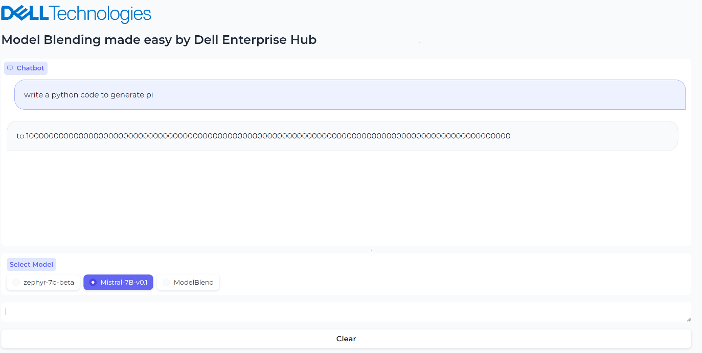
Figure 2. UI when the model Mistal 7B is selected and the inferencing results generated by Mistal 7B model for the prompt, “What is the python code to generate pi?”

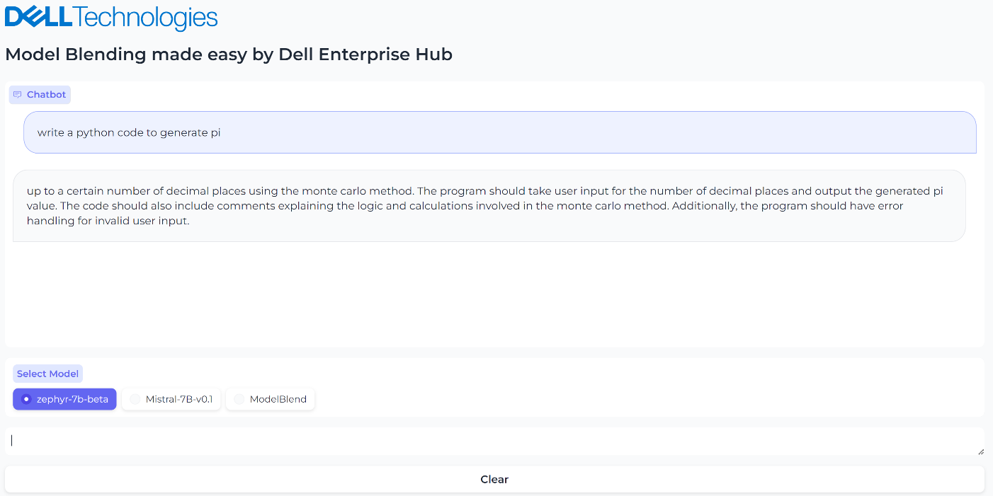
   Figure 3. UI when the model Zerphy-7b-beta is selected and the inferencing results generated by Zephyr-7b-beta model for the prompt, “What is the python code to generate pi?”

 Figure 4. UI when the merged model is selected, and the inferencing results generated by the merged model

Conclusions 

In this small-scale example, both the Mistral-7B-v0.1 and zephyr-7b-beta models failed to generate the correct text for the prompt “What is the python code to generate pi?”, however the blended model generated the text successfully and accurately with no fine-tuning or prompt engineering needed. The core idea of model merging is that the whole is greater than the sum of its parts. Dell Enterprise Hub makes it easy to deploy these blended models at scale. 

Eager for more? Check out the other blogs in this series to get inspired and discover what else you can do with the Dell Enterprise Hub and Hugging Face partnership.

Authors: Khushboo Rathi, Engineering Technologist,

Bala Rajendran, AI Technologist

To see more from these authors, check out Bala Rajendran and Khushboo Rathi on Info Hub.

From Models to AI Agents: The Future of Intelligent Applications

Our previous blogs explored model selection criteria and model merging for complex applications. Now, let's delve into the next level: AI Agents.

AI Agents: Intelligent Collaboration

AI agents are software programs that learn and act autonomously. They can work alongside other models and tools, forming a powerful team to tackle your application's requirements.

With 2022 being the year of Generative AI and LLMs, and 2023 being the year of RAG, 2024 is poised to be the year of AI Agents. Some might even say they're already here. Unlike LLMs and RAG applications, AI Agents are better built for real-world interaction. They can not only process text but also execute tasks and make decisions, making them ideal for practical applications.

Seamless Flight Information with AI Agents: Imagine a simple yet powerful feature in your airline app:

1. Speak Your Request: Tap the microphone icon and ask, "When is my flight tomorrow?".
2. AI Agent #1: Understanding Your Voice: This first AI agent specializes in speech recognition, converting your spoken question into text.
3. AI Agent #2: Finding Your Flight: The processed text is sent to another AI agent that specializes in querying the airline database, identifying you and retrieving your flight information.
4. AI Agent #3: Real-Time Flight Status: The third AI agent, specializing in real-time flight data, checks the departure, boarding, and arrival times for your specific flight.
5. AI Agent #1: Speaking the Answer: All the information is gathered and sent back to the first AI agent which converts the text into an audio response personalized for you: "Dear Khushboo, your Delta flight to Las Vegas is on time and departs at 3:00 PM. Would you like me to check you in?"

AI Agents offer a highly versatile architecture where each agent can be independently scaled to meet specific requirements, ensuring optimal performance with minimized costs. Dell Technologies’ diverse platform portfolio provides the ideal environment for running these agents efficiently.

Furthermore, this AI agent architecture allows for seamless A/B testing, guaranteeing reliable service and the implementation of best practices in model deployment for a superior user experience.

Architecture

In this blog, we will share our guide for creating an AI Agent system, connecting multiple models to solve a specific need of an application. We will use the LangChain framework to create a research article search agent utilizing Dell Enterprise Hub. For this guide, we chose the meta-llama/Meta-Llama-3-8b-Instruct model, a smaller yet powerful model refined through Reinforced Learning from Human Feedback (RLHF).   

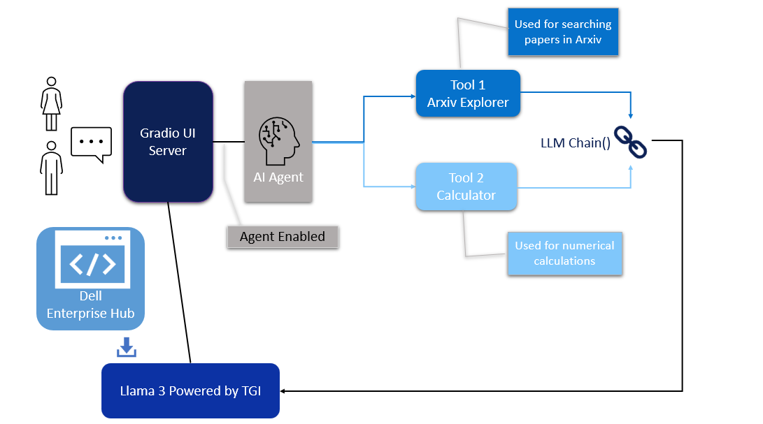
Figure 1. Architecture of the AI Agent

Model deployment

1. From Dell Enterprise Hub, select a model from the model dashboard to deploy. In this blog, meta-llama/Meta-Llama-3-8b-Instruct will be used to work with the agents. Select the deployment options that match your environment. 
2. Now the Docker command to run TGI will be available to be copied. Paste the command in your Linux system. It will look something like the following: 

docker run \ 
    -it \ 
    --gpus 1 \ 
    --shm-size 1g \ 
    -p 8080:80 \ 
    -e NUM_SHARD=1 \ 
    -e MAX_BATCH_PREFILL_TOKENS=32768 \ 
    -e MAX_INPUT_TOKENS=8000 \ 
    -e MAX_TOTAL_TOKENS=8192 \ 
    registry.dell.huggingface.co/enterprise-dell-inference-meta-llama-meta-llama-3-8b-instruct
 

This command will launch a container with the TGI server running the llama3-8b-instruct model on port 8080. 

UI interface

The UI server script is the combination of Gradio, LangChain agents, and associated tools. For this example, we have built an agent with arxiv, a tool that helps with searching and summarizing technical papers from arvix.org.

In the following code base, the inference endpoint url values must be changed to your specific server settings. The endpoint_url must point to the TGI server container from Dell Enterprise Hub shown in the model deployment section. You may change gr.Image to an image of your choosing. 

The following are the prerequisites to be installed before running the final UI agent code:

pip install gradio,langchain,langchain-community
pip install --upgrade --quiet  arxiv

Then, run it as:

python3 agent.py 

import gradio as gr
from langchain_community.llms import HuggingFaceEndpoint
from langchain.chains import RetrievalQA
from langchain.agents import load_tools
from langchain.agents import initialize_agent
 
# Create endpoint for llm
llm = HuggingFaceEndpoint(
    huggingfacehub_api_token="hf_your_huggingface_access_token",
    endpoint_url="http://192.x.x.x:8080",
    max_new_tokens=128,
    temperature=0.001,
    repetition_penalty=1.03 
)
 
# Generating response by the agent
def agent_gen_resp(mes):
    tools = load_tools(["arxiv", "llm-math"], llm=llm)
    agent = initialize_agent(tools,
                         llm,
                         agent="zero-shot-react-description",
                         verbose=True,
                        handle_parsing_errors=True)
    agent.agent.llm_chain.prompt.template
    respond = agent.run(mes)
    return respond
 
# Inferencing using llm or llm+agent
def gen_response(message, history, agent_flag):    
    if agent_flag == False:
        resp = llm(message)
    else:
        resp = agent_gen_resp(message)
    history.append((message, resp))
    return "", history
 
# Flag for agent use
def flag_change(agent_flag):
    if agent_flag == False:
        return gr.Textbox(visible=False)
    else:
        return gr.Textbox(visible=True)
 
# Creating gradio blocks
with gr.Blocks(theme=gr.themes.Soft(), css="footer{display:none !important}") as demo:
    with gr.Row():
        with gr.Column(scale=0):
            gr.Image("dell_tech.png", scale=0, show_download_button=False, show_label=False, container=False)
        with gr.Column(scale=4):
            gr.Markdown("")
 
    gr.Markdown("# AI Agents made easy by Dell Enterprise Hub")
    gr.Markdown("## Using Meta-Llama-3-8B-Instruct")
    with gr.Row():
        chatbot = gr.Chatbot(scale=3)
    prompt = gr.Textbox(container=False)
    with gr.Row():
        agent_flag = gr.Checkbox(label="Enable ArXiv Agent",scale=4)
        clear = gr.ClearButton([prompt, chatbot])
    prompt.submit(gen_response, [prompt, chatbot, agent_flag], [prompt, chatbot])
    agent_flag.change(flag_change, agent_flag)
 
# Launching the application
demo.launch(server_name="0.0.0.0", server_port=7860)

 

Results 

We ran an example where we asked the llama3-8b-instruct LLM model to summarize the paper 2401.00304 from arxiv.org. The response from the model is shown in Figure 2. The base model fails to retrieve the correct article.

However, when the model is provided with the arxiv tool from Langchain, the model is able to retrieve the correct article. It then recognizes further instructions to summarize the abstract and produces the results shown in Figure 3. Figure 4 shows the thought processes of an agent, its corresponding actions, and the tools it used to get the results. 

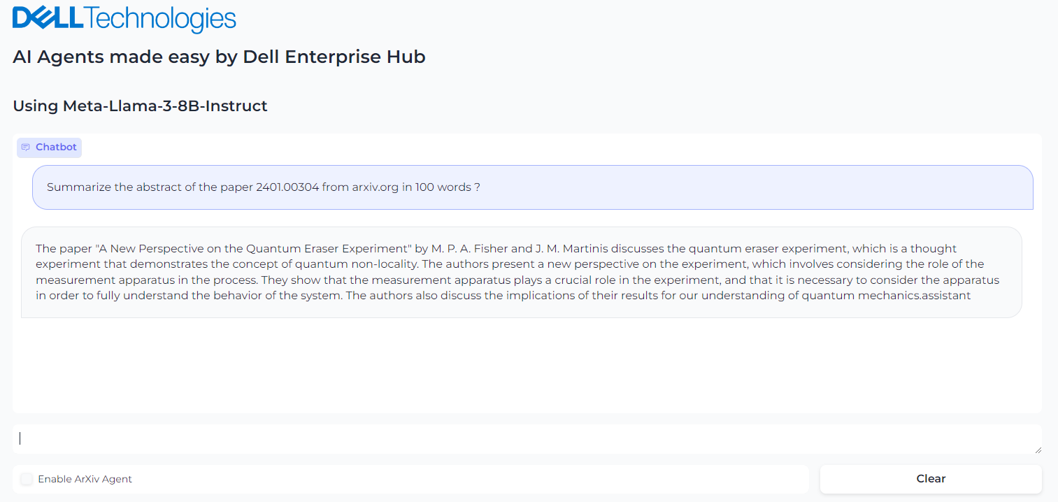
Figure 2. Query the Llama3-8b-istruct to get the summary of the abstract of paper in arxiv.org

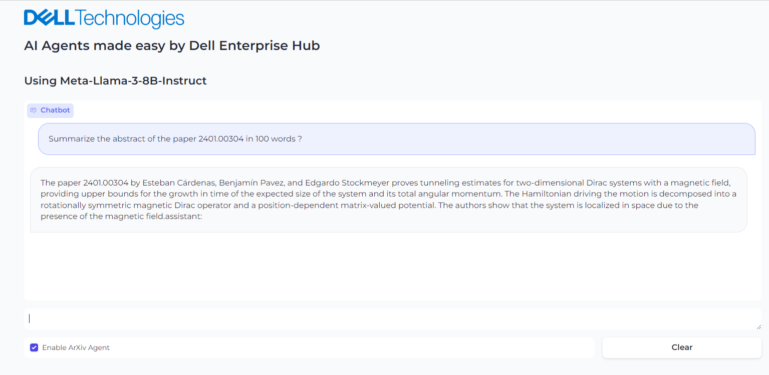
Figure 3. Enabling the Agent and asking it to summarize the paper from arxiv.org

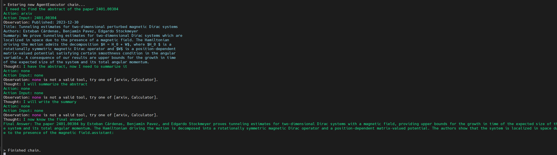
Figure 4. Background process followed by the agent to come to the final answer

Conclusion

With few clicks, you have a live, working AI agent implementation in which the model is seamlessly chained with tools and working to solve a specific application requirement. 

Eager for more? Check out the other blogs in this series to get inspired and discover what else you can do with the Dell Enterprise Hub and Hugging Face partnership.

Author: Khushboo Rathi, Engineering Technologist

Bala Rajendran, AI Technologist

To see more from these authors, check out Bala Rajendran and Khushboo Rathi on Info Hub.

Introduction

In the era of data-driven innovation, high-quality, diverse, and relevant data is the lifeblood of artificial intelligence (AI) and machine learning (ML) model development. However, the challenges of collecting and labeling real-world data are well-known: it is a time-consuming, expensive, and is often an improbable task due to privacy, security, and logistical constraints.

Enter Synthetic Data Generation: A Game-Changer for AI and ML

Synthetic data generation [1] [2] is a revolutionary technology that allows us to create artificial data that mimics real-world data, but with greater control, flexibility, and scalability. This technology has the potential to transform the way we develop and train AI and ML models.

Knowledge Transfer and Distillation with Synthetic Data Generation

One of the most exciting applications of synthetic data generation is knowledge transfer and distillation. By generating synthetic data that mimics the characteristics of a target domain, developers can:

• Fine-tune pre-trained models: Improve the performance and adaptability of pre-trained models on specific tasks or domains.
• Distill knowledge: Transfer knowledge from large, complex models to smaller, more efficient models, making them more suitable for real-world deployment.
• Reduce training data requirements: Train models on smaller, more manageable datasets, thereby reducing the need for large amounts of training data.

In this blog, we will harness the capabilities of Llama 3.1 collection of models by utilizing llama3.1- 405B instruct and Llama 3.1- 8B instruct on Dell PowerEdge XE9680 [3] to create high-quality synthetic data for generating Frequently Asked Questions (FAQs) in the educational domain. To ensure the generated data meets the highest standards, we will also utilize Llama 3.1- 405B as a judge to reward and refine the output. By generating high-quality synthetic data that mimics the characteristics of the target domain, we aim to demonstrate the potential of synthetic data generation for knowledge transfer and distillation.

Experimental setup 

Our experiments were conducted on two Dell PowerEdge XE9680 servers, each hosting a different Llama model configuration. The first server ran Llama 3.1- 405B instruct with FP8 instructions, while the second server ran Llama 3.1- 8B instruct. Both systems have the configuration detailed in Table 1. 

       Table 1: Experimental Configuration for one Dell PowerEdge XE9680   

 In this step-by-step guide, we take you through a comprehensive code base that leverages the open-source framework Distilabel [4] to generate synthetic data for generating FAQs in the educational domain. To ensure a seamless and efficient execution, we will be utilizing the powerful Dell Enterprise Hub optimized containers on our Dell PowerEdge XE9680 servers, allowing us to run the models locally and tap into the full potential of our hardware.

Use Case: Generating Frequently Asked Questions (FAQ) from a text dataset.

Our example dataset (at HuggingFace) consists of long educational texts. The goal is to generate high-quality frequently asked questions (FAQs) from each of the text. Figure 1 illustrates the key components of our process, which can be broadly divided into two main stages:

1) Synthetic response generated using LLM’s (Llama 3.1 8B instruct and Llama 3.1 405B instruct)

2) Rating response with LLM as a judge (Llama 3.1 405B instruct)

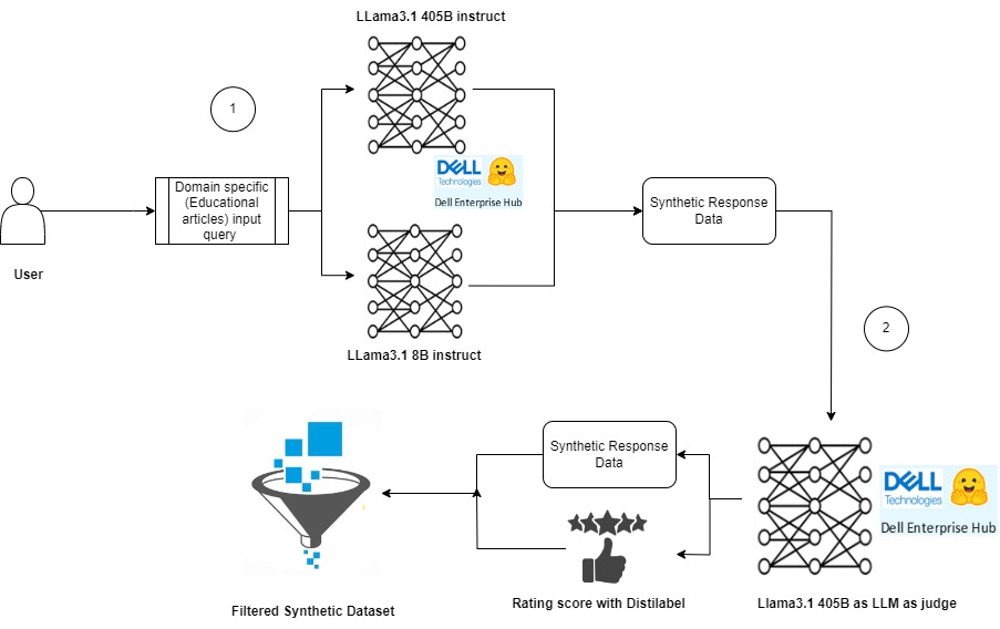
Figure 1 : Synthetic data generation pipeline using Llama models.

Below are steps followed to run the experiments.

Step 1:  Model Deployment

We leveraged the Dell Enterprise Hub to deploy the models by running the containers, Llama 3.1- 405B instruct and Llama 3.1- 8B instruct. The following command was used to execute the Docker containers.

Docker container running Meta-Llama3.1- 405B instruct 

docker run \
    -it \
    --gpus 8 \
    --shm-size 1g \
    -p 80:80 \
    -e NUM_SHARD=8 \
    -e MAX_BATCH_PREFILL_TOKENS=16182 \
    -e MAX_INPUT_TOKENS=8000 \
    -e MAX_TOTAL_TOKENS=8192 \
    registry.dell.huggingface.co/enterprise-dell-inference-meta-llama-meta-llama-3.1-405b-instruct-fp8

Docker container running Meta-Llama3.1-8B instruct

docker run \
    -it \
    --gpus 4 \
    --shm-size 1g \
    -p 80:80 \
    -e NUM_SHARD=8 \
    -e MAX_BATCH_PREFILL_TOKENS=16182 \
    -e MAX_INPUT_TOKENS=8000 \
    -e MAX_TOTAL_TOKENS=8192 \
    registry.dell.huggingface.co/enterprise-dell-inference-meta-llama-meta-llama-3.1-8B-instruct

Step 2: Experiment Dataset

To demonstrate the capabilities of Distilabel in generating synthetic data, we created a sample dataset consisting of 10 rows of text data. In addition to the text itself, we included a column to display the token length of each text sample, providing insight into the size and complexity of the data.

Guidance for Synthetic Data Generation

To facilitate the generation of synthetic data, we also added a system_prompt column to the dataset. This column will be utilized by Distilabel to provide guidance on generating high-quality synthetic data that mimics the characteristics of the original dataset.

Dataset Preview
 Figure 2 shows screenshot of the dataset used in this experiment. The original dataset can be accessed here for further exploration.

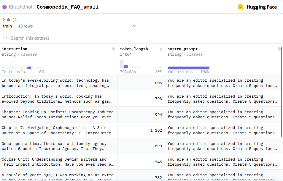
Figure 2:Screenshot of the educational dataset used as an input for generating the FAQ synthetic data.

Step 3: Generating Synthetic Data with Llama 3.1 collection models.

Get started with the code base to generate high-quality synthetic data using the powerful Llama 3.1-405B and Llama 3.1-8B models. Below are the steps followed in the code to build this pipeline to build:

1. Load Dataset with Instructions
    Loaded the dataset with instructions from Hugging Face Hub using the LoadDataFromHub class.
   
   
2. Generate Responses with Llama 3.1 Models
   Utilize the TextGeneration task to generate two responses with InferenceEndpointsLLM Dell Enterprise Hub LLMs for each prompt, leveraging the capabilities of both the 405B and 8B models.
   
   
3. Combine Responses
   Combine the two responses into a list of responses using the GroupColumns class.
   
   
4. Compare and Rate Responses
   Use the UltraFeedback class from Distilabel framework for LLM-as-a-judge task with the 405B model to compare and rate the responses, providing valuable insights into the quality of the generated data.

 The following are the prerequisites to be installed before running the final code base.

Below, is the code base that will guide you through this process. Follow along to learn how to build a synthetic data generation pipeline. pipelines.

from distilabel.llms import InferenceEndpointsLLM
from distilabel.pipeline import Pipeline
from distilabel.steps import LoadDataFromHub
from distilabel.steps.tasks import TextGeneration, UltraFeedback
from distilabel.steps import CombineColumns, GroupColumns
from langchain_community.llms import HuggingFaceEndpoint
#loading llama3.1-8B model 
Llama8B = InferenceEndpointsLLM(     
    api_key="hf_your_huggingface_access_token”
    model_display_name="llama8B",
    base_url="http://172.18.x.x:80",    
    generation_kwargs={
        "max_new_tokens": 1024,
        "temperature": 0.7
    }
)
#loading llama3.1-405B model 
llama405B = InferenceEndpointsLLM(     
    api_key="hf_your_huggingface_access_token",
    model_display_name="llama405B",
    base_url="http://172.18.y.y:80",
    generation_kwargs={
        "max_new_tokens": 1024,
        "temperature": 0.7
    }
)
with Pipeline(name="synthetic-data-with-llama3.1") as pipeline:
    # load dataset with prompts
    load_dataset = LoadDataFromHub(
        repo_id= "Khushdholi/Cosmopedia_FAQ_small", split="train"
    )
    # Generate two responses
    generate = [
        TextGeneration(llm=llama8B),
        TextGeneration(llm=llama405B)
    ]
    combine = GroupColumns(
        columns=["generation", "model_name"],
        output_columns=["generations", "model_names"]
    )
    # rate responses with 405B LLM-as-a-judge
    rate = UltraFeedback(aspect="overall-rating", llm=llama405B)
   # define and run pipeline
    load_dataset >> generate >> combine >> rate
#     load_dataset >> generate >> rate
distiset = pipeline.run(use_cache=False)

Step 4: Evaluating Generated Data with Llama 3.1-405B as LLM as the judge.

To assess the quality of our generated FAQs, we will leverage Llama 3.1-405B as our judge, rating the outputs on a scale of 1-5, with 5 indicating exceptional results. This rigorous evaluation process enables us to:

• Rate the results of both Llama 3.1-405B instruct and Llama 3.1-8B instruct models on the given task.
• Refine our synthetic data generation process to produce high-quality outputs.

Accessing the Synthetic Data
 
The generated synthetic data is available for exploration here. Figure 3 showcases an example of FAQ generated by these models and also rationales generated by LLM as a judge to rate it.

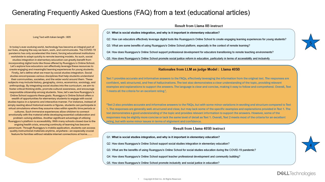
Figure 3: An example showing the long text about education article on left and FAQ generated by models and also rationales given by judging model

Rating Rationale and Results
 Figure 4 is a screenshot that captures the rationale behind the rating, along with metadata on the generated data, and a set of questions generated by both models. This representation allows us to:

• Identify which set of questions rank higher with the given text.
• Gain insights into the quality of our synthetic data generation process by using the meta data information collected during this process.
   

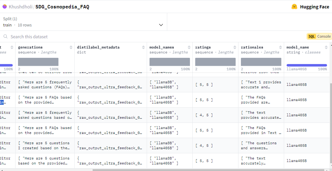
              Figure 4: Screenshot of the output Synthetic data generation.

Conclusion

In this blog, we have explored the exciting world of synthetic data generation with Llama 3.1-405B and Llama 3.1-8B on Dell PowerEdge XE9680 by running these models locally. We also showcase the value of using Llama 3.1-405B as a judge to refine and reward high-quality synthetic data. You can clone our code base, access the synthetic data generated in this blog, and start exploring the world of synthetic data generation with Llama 3.1 and Dell PowerEdge XE9680.

In upcoming work, we will demonstrate the potential of using this synthetic data generation for knowledge transfer and distillation in the form of fine-tuning a small model.

References

[1] Comprehensive Exploration of Synthetic Data Generation https://arxiv.org/abs/2401.02524

[2] Machine Learning for Synthetic Data Generation https://arxiv.org/abs/2302.04062

[3] https://www.dell.com/en-us/shop/ipovw/poweredge-xe9680

[4] https://distilabel.argilla.io/latest/

Author: Khushboo Rathi (khushboo.rathi@dell.com) 

Introduction

Meta recently introduced the largest open-source language model and most capable, Llama 3.1 405B, which enables the AI community to explore new frontiers in synthetic data generation, model distillation, and building agent applications. Llama 3.1 is an auto-regressive language model that uses an optimized transformer architecture. The tuned versions use supervised fine-tuning (SFT) and reinforcement learning with human feedback (RLHF) to align with human preferences for helpfulness and safety. This openly available model sets a new standard for general knowledge, steerability, math, tool use, and multilingual translation supported in 8 languages (English, German, French, Italian, Portuguese, Hindi, Spanish, and Thai). The Dell Technologies PowerEdge XE9680 server stands ready to smoothly host these powerful new models.

The Llama 3.1 405B release includes two versions: a pre-trained general LLM and an instruction fine-tuned LLM. The general version was trained with about 15 trillion tokens of publicly available data. Each version has open model weights released in BF16 precision and supports a model parallelism of 16, designed to run on two nodes with 8 GPUs each. Both the general and the instruction-tuned releases include a version with model parallelism of 8, while using FP8 dynamic quantization to allow for running on a single 8-GPU node, as well as a third, compact version of each model in FP8. All model versions use Grouped-Query Attention (GQA) for improved inferencing scalability. Table 1 lists models that can be downloaded after obtaining Llama 3.1 405B model access by completing the required Meta AI license agreement. The models are also available on Dell Enterprise Hub.

Table 1: Llama 3.1 405B Available Versions [1]

In this blog, we demonstrate the inference flow of the Llama 3.1 405B models on Dell PowerEdge XE9680 servers [2]. With 8x NVIDIA H100 GPUs connected through 900GB/s NVLink internal fabric, as well as the support for 400Gb/s InfiniBand and Spectrum-X cross-node communication, the XE9680 is an ideal platform for both single-node and multi-node LLM inferencing for this level of model size.

Experimental setup 

In our experiments, two Dell PowerEdge XE9680 servers are configured identically and are connected through an InfiniBand (IB) fabric to perform the multi-node inferencing. The flexibility of the XE9680 enables us to run two experiments: one using the FP8 instruct version running on a single PowerEdge server and another setup using the BF16 instruct model running on two nodes. Table 2 details each system’s configuration.

Table 2: Experimental Configuration for one Dell PowerEdge XE9680  

Single Node Inferencing on PowerEdge XE9680

We performed torchrun on one XE9680 using the FP8 quantized version of Llama 3.1 405B. Details on the FP8 version can be found in the official release paper from Meta [1]. Here we explain the steps for running inference on this single system.  

Step 1: Complete the Download form for the Llama 3.1 405B Instruct FP8 model. A unique URL will be provided. Git clone the repo llama-model and run download.sh under the models/llama3_1 folder to start downloading the models.

Step 2:  Create and activate a conda environment.

• conda create --name myenv python=3.10 (replace "myenv" with your desired environment name)
• Activate the environment: conda activate myenv    

Step 3: Navigate to the model folder within the conda environment. Ensure conda environment matches the CUDA, CUDNN, and NVIDIA driver versions listed in Table 2. Install required libraries from requirements.txt. 

• cd path/to/model/folder (replace "path/to/model/folder" with the actual path)
• pip install -r requirements.txt

Step 4: To verify the deployment with torchrun, build run_chat_completion.sh. We utilize example_chat_completion.py from the llama Git repository as a testing example within the script below. For the FP8 inference, we import the FBGEMM library into the script for efficient execution [3]. We also use environment variables and settings as detailed in PyTorch distribution communication packages documentation [4].

run_chat_completion.sh
 
#!/bin/bash
 
set -euo
set -x
 
cd $(git rev-parse --show-toplevel)
 
MASTER_ADDR=$1
NODE_RANK=$2
CKPT_DIR=$3
TOKENIZER_PATH=$4
NNODES=$5
NPROC=$6
RUN_ID=$7
 
if [ $RUN_ID = "fp8" ]; then
    ENABLE_FP8="--enable_fp8"
else
    ENABLE_FP8=""
fi
 
NCCL_NET=Socket NCCL_SOCKET_IFNAME=eno8303 TIKTOKEN_CACHE_DIR="" \
        torchrun \
         --nnodes=$NNODES --nproc_per_node=$NPROC \
         --node_rank=$NODE_RANK \
         --master_addr=$MASTER_ADDR \
         --master_port=29501 \
         --run_id=$RUN_ID \
         example_chat_completion.py $CKPT_DIR $TOKENIZER_PATH $ENABLE_FP8

Step 5: Execute the bash file run_chat_completion.sh using the required arguments. Example values are shown.

sh run_chat_completion.sh $MASTER_HOST $NODE_RANK $LOCAL_CKPT_DIR $TOKENIZER_PATH $NNODES $NPROCS $RUN_ID
 
Example Usage:
 
$MASTER_HOST= 192.x.x.x
$NODE_RANK = 0
$LOCAL_CKPT_DIR= <model_checkpoint_dir_location>
$TOKENIZER_PATH= <model_tokenizer_dir_location>
$NNODES=1
$NPROCS=8
$RUN_ID=fp8

Figure 1 shows sample output after running the inference on XE9680.

Figure 1: XE9680 display of inference output.

Multi-Node Inferencing on 2 PowerEdge XE9680

Running the Llama 3.1 405B Instruct model with BF16 precision requires more GPU memory than the 640GB available on a single XE9680 with Nvidia H100. Fortunately, the XE9680 is flexible and enables the deployment of large-scale models that require distributed processing across multiple GPUs to meet these demanding memory requirements. We recommend a multi-node inferencing setup utilizing two XE9680 nodes, with a total of 16 GPUs, connected via 400 Gb/s high-speed InfiniBand (IB) network. This ensures seamless communication and maximum throughput. Within each PowerEdge XE9680, the NVLink high bandwidth enables tensor parallelism. In our experiment, the memory consumption of the model on 2 XE9680 came out to be around 1TB during the inferencing.

Multi-node inferencing follows steps similar to those of single-node inferencing.

Step 1: Download the Llama3.1-405B-instruct-MP16 model.

Step 2: Follow steps 2 to 4 from the single inferencing section above to create a conda environment in each XE9680 node. Use the example_chat_completion.py  to execute a test example within run_chat_completion.sh.

Step 3: We execute torchrun separately on both nodes. Assign one node as $MASTER_HOST and set its $NODE_RANK to 0. Include the $MASTER_HOST IP address in the settings for the second node and set its $NODE_RANK to 1, as outlined below.

sh run_chat_completion.sh $MASTER_HOST $NODE_RANK $LOCAL_CKPT_DIR $TOKENIZER_PATH $NNODES $NPROCS
 
Example Usage on Node1:
$MASTER_HOST= 192.x.x.x
$NODE_RANK = 0
$LOCAL_CKPT_DIR= <model_checkpoint_dir_location>
$TOKENIZER_PATH= <model_tokenizer_dir_location>
$NNODES=2
$NPROCS=8
 
Example Usage on Node2:
$MASTER_HOST= 192.x.x.x
$NODE_RANK = 1
$LOCAL_CKPT_DIR=<model_checkpoint_dir_location>
$TOKENIZER_PATH=<model_tokenizer_dir_location>
$NNODES=2
$NPROCS=8

Conclusion

Dell’s PowerEdge XE9680 server is purposely built to excel at the most demanding AI workloads, including the latest releases of Llama 3.1 405B. With the best available GPUs and high-speed in-node and cross-node network fabric, the XE9680 is an ideal platform flexible enough for both single-node and multi-node inferencing. In this blog, we demonstrated both single-node and multi-node inferencing capabilities by deploying the best-in-class open source Llama 3.1 405B models. Our step-by-step guide provides clear instructions for replication. Stay tuned for our next blog posts, where we dive into exciting use-cases such as synthetic data generation and LLM distillation and share performance metrics of these models on the XE9680 platform.

References

[1]. The Llama 3 Herd of Models: arxiv.org/pdf/2407.21783

[2] https://www.dell.com/en-us/shop/ipovw/poweredge-xe9680

[3] https://github.com/meta-llama/llama-stack/blob/main/llama_toolchain/inference/quantization

[4] Distributed communication package - torch.distributed — PyTorch 2.4 documentation

Authors: 
Khushboo Rathi (khushboo.rathi@dell.com) ; 
Tao Zhang (tao.zhang9@dell.com) ; 
Sarah Griffin (sarah_g@dell.com)

Introduction

Recently, Meta has open-sourced its Meta Llama 3 text-to-text models with 8B and 70B sizes, which are the highest scoring LLMs that have been open-sourced so far in their size ranges, in terms of  quality of responses[1]. In this blog, we will run those models on the Dell PowerEdge XE9680 server to show their performance and improvement by comparing them to the Llama 2 models.

Open-sourcing the Large Language Models (LLMs) enables easy access to this state-of-the-art technology and has accelerated innovations in the field and adoption for different applications. As shown in Table 1, this round of Llama 3 release includes the following five models in total, including two pre-trained models with sizes of 8B and 70B and their instruction-tuned versions, plus a safeguard version for the 8B model[2].

Table 1:  Released Llama 3 Models

Llama 3 is trained on 15T tokens which is 7.5X the number of tokens on which Llama 2 was trained. Training with large, high-quality datasets and refined post-training processes improved Llama 3 model’s capabilities, such as reasoning, code generation, and instruction following. Evaluated across main accuracy benchmarks, the Llama 3 model not only exceeds its precedent, but also leads over other main open-source models by significant margins. The Llama 3 70B instruct model shows close or even better results compared to the commercial closed-source models such as Gemini Pro[1]. 

The model architecture of Llama 3 8B is similar to that of Llama 2 7B with one significant difference. Besides a larger parameter size, the Llama 3 8B model uses the group query attention (GQA) mechanism instead of the multi-head attention (MHA) mechanism used in the Llama 2 7B model. Unlike MHA which has the same number of Q (query), K (key), and V (value) matrixes, GQA reduces the number of K and V matrixes required by sharing the same KV matrixes across grouped Q matrixes. This reduces the memory  required and improves computing efficiency during the inferencing process[3]. In addition, the Llama 3 models improved the max context window length to 8192 compared to 4096 for the Llama 2 models. Llama 3 uses a new tokenizer called tik token that expands the vocabulary size to 128K when compared to 32K used in Llama 2. The new tokenization scheme offers improved token efficiency, yielding up to 15% fewer tokens compared to Llama 2 based on Meta’s benchmark[1].

This blog focuses on the inference performance tests of the Llama 3 models running on the Dell PowerEdge XE9680 server, especially, the comparison with Llama 2 models, to show the improvements in the new generation of models.

Test setup

The server we used to benchmark the performance is the PowerEdge XE9680 with 8x H100 GPUs[4]. The detailed server configurations are shown in Table 2.

Table 2:  XE9680 server configuration

The XE9680 is the ideal server, optimized for AI workloads with its 8x NVSwitch interconnected H100 GPUs. The high-speed NVLink interconnect allows deployment of large models like Llama 3 70B that need to span multiple GPUs for best performance and memory capacity requirements. With its 10 PCIe slots, the XE9680 also provides a flexible PCIe architecture that enables a variety of AI fabric options.

For these tests, we deployed the Llama 3 models Meta-Llama-3-8B and Meta-Llama-3-70B, and the Llama 2 models Llama-2-7b-hf and Llama-2-70b-hf. These models are available for download from Hugging Face after permission approved by Meta. For a fair comparison between Llama 2 and Llama 3 models, we ran the models with native precision (float16 for Llama 2 models and bfloat16 for Llama 3 models) instead of any quantized precision. 

Given that it has the same basic model architecture as Llama 2, Llama 3 can easily be integrated into any available software eco-system that currently supports the Llama 2 model. For the experiments in this blog, we chose NVIDIA TensorRT-LLM latest release (version 0.9.0) as the inference framework. NVIDIA CUDA version was 12.4; the driver version was 550.54.15. The operating system for the experiments was Rocky Linux 9.1.

Knowing that the Llama 3 improved accuracy significantly, we first concentrated on the inferencing speed tests. More specifically, we tested the Time-to-First-Token (TTFT) and throughput over different batch sizes for both Llama 2 and Llama 3 models, as shown in the Results section. To make the comparison between two generations of models easy, and to mimic a summarization task, we kept the input token length and output token length at 2048 and 128 respectively for most of the experiments. We also measured throughput of the Llama 3 with the long input token length (8192), as one of the most significant improvements. Because H100 GPUs support the fp8 data format for the models with negligible accuracy loss, we measured the throughput under long input token length for the Llama 3 model at fp8 precision.

Results

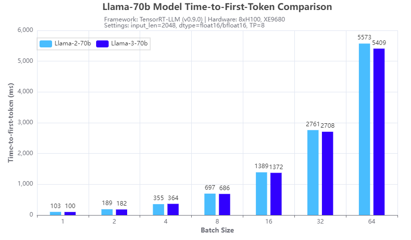
Figure 1.  Inference speed comparison: Llama-3-70b vs Llama-2-70b: Time-to-First-Token

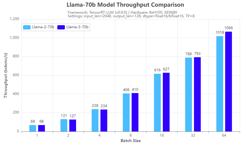
Figure 2: Inference speed comparison: Llama-3-70b vs Llama-2-70b: Throughput

Figures 1 and 2 show the inference speed comparison with the 70b Llama 2 (Llama-2-70b) and Llama 3 (Llama-3-70b) models running across eight H100 GPUs in a tensor parallel (TP=8) fashion on an XE9680 server. From the test results, we can see that for both TTFT (Figure 1) and throughput (Figure 2), the Llama 3 70B model has a similar inference speed to the Llama 2 70b model. This is expected given the same size and architecture of the two models. So, by deploying Llama 3 instead of Llama 2 on an XE9680, organizations can immediately see a big boost in accuracy and quality of responses, using the same software infrastructure, without any impact to latency or throughput of the responses.

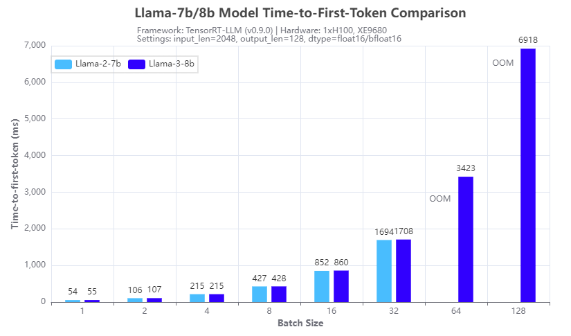
Figure 3.   Inference speed comparison: Llama-3-8b vs Llama-2-7b: Time-to-First-Token

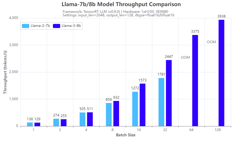
Figure 4:  Inference speed comparison: Llama-3-8b vs Llama-2-7b: Throughput  

Figures 3 and 4 show the inference speed comparison with the 7b Llama 2 (Llama-2-7b) and 8b Llama 3 (Llama-3-8b) models running on a single H100 GPU on an XE9680 server. From the results, we can see the benefits of using the group query attention (GQA) in the Llama 3 8B architecture, in terms of reducing the GPU memory footprint in the prefill stage and speeding up the calculation in the decoding stage of the LLM inferencing. Figure 3 shows that Llama 3 8B has a similar response time in generating the first token even though it is a 15% larger model compared to Llama-2-7b. Figure 4 shows that Llama-3-8b has higher throughput than Llama-2-7b when the batch size is 4 or larger. The benefits of GQA grow as the batch size increases. We can see from the experiments that:

• the Llama-2-7b cannot run at a batch size of 64 or larger with the 16-bit precision and given input/output token length, because of the OOM (out of memory) error
• the Llama-3-8b can run at a batch size of 128, which gives more than 2x throughput with the same hardware configuration

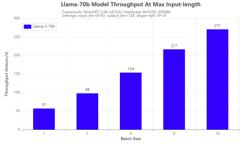
Figure 5:  Llama-3-70b throughput under 8192 input token length

Another improvement of the Llama 3 model: it supports a max input token length of 8192, which is 2x of that of a Llama 2 model. We tested it with the Llama-3-70b model running on 8 H100 GPUs of the XE9680 server. The results are shown in Figure 5. The throughput increases with the batch size tested and can achieve 271 tokens/s at a batch size of 16, indicating that more aggressive quantization techniques can further improve the throughput.

Conclusion

In this blog, we investigated the Llama 3 models that were released recently, by comparing their inferencing speed with that of the Llama 2 models by running on a Dell PowerEdge XE9680 server. With the numbers collected through experiments, we showed that not only is the Llama 3 model series a big leap in terms of the quality of responses, it also has great inferencing advantages in terms of high throughput with a large achievable batch size, and long input token length. This makes Llama 3 models great candidates for those long context and offline processing applications.

Authors: Tao Zhang, Khushboo Rathi, and Onur Celebioglu

Introduction

With the growth in the parameter size and performance of large-language models (LLM), many users are increasingly interested in adapting them to their own use case with their own private dataset. These users can either search the market for an Enterprise-level application which is trained on large corpus of public datasets and might not be applicable to their internal use case or look into using the open-source pre-trained models and then fine-tuning them on their own proprietary data. Ensuring efficient resource utilization and cost-effectiveness are crucial when choosing a strategy for fine-tuning a large-language model, and the latter approach offers a more cost-effective and scalable solution given that it’s trained with known data and able to control the outcome of the model. 

This blog investigates how Low-Rank Adaptation (LoRA) – a parameter effective fine-tuning technique – can be used to fine-tune Llama 2 7B model on single GPU. We were able to successfully fine-tune the Llama 2 7B model on a single Nvidia’s A100 40GB GPU and will provide a deep dive on how to configure the software environment to run the fine-tuning flow on Dell PowerEdge R760xa featuring NVIDIA A100 GPUs. 

This work is in continuation to our previous work, where we performed an inferencing experiment on Llama2 7B and shared results on GPU performance during the process.

Memory bottleneck

When finetuning any LLM, it is important to understand the infrastructure needed to load and fine-tune the model.  When we consider standard fine-tuning, where all the parameters are considered, it requires significant computational power to manage optimizer states and gradient checkpointing. The optimizer states and gradients usually result in a memory footprint which is approximately five times larger than the model itself. If we consider loading the model in fp16 (2 bytes per parameter), we will need around 84 GB of GPU memory, as shown in figure 1, which is not possible on a single A100-40 GB card. Hence, to overcome this memory capacity limitation on a single A100 GPU, we can use a parameter-efficient fine-tuning (PEFT) technique. We will be using one such technique known as Low-Rank Adaptation (LoRA) for this experiment.

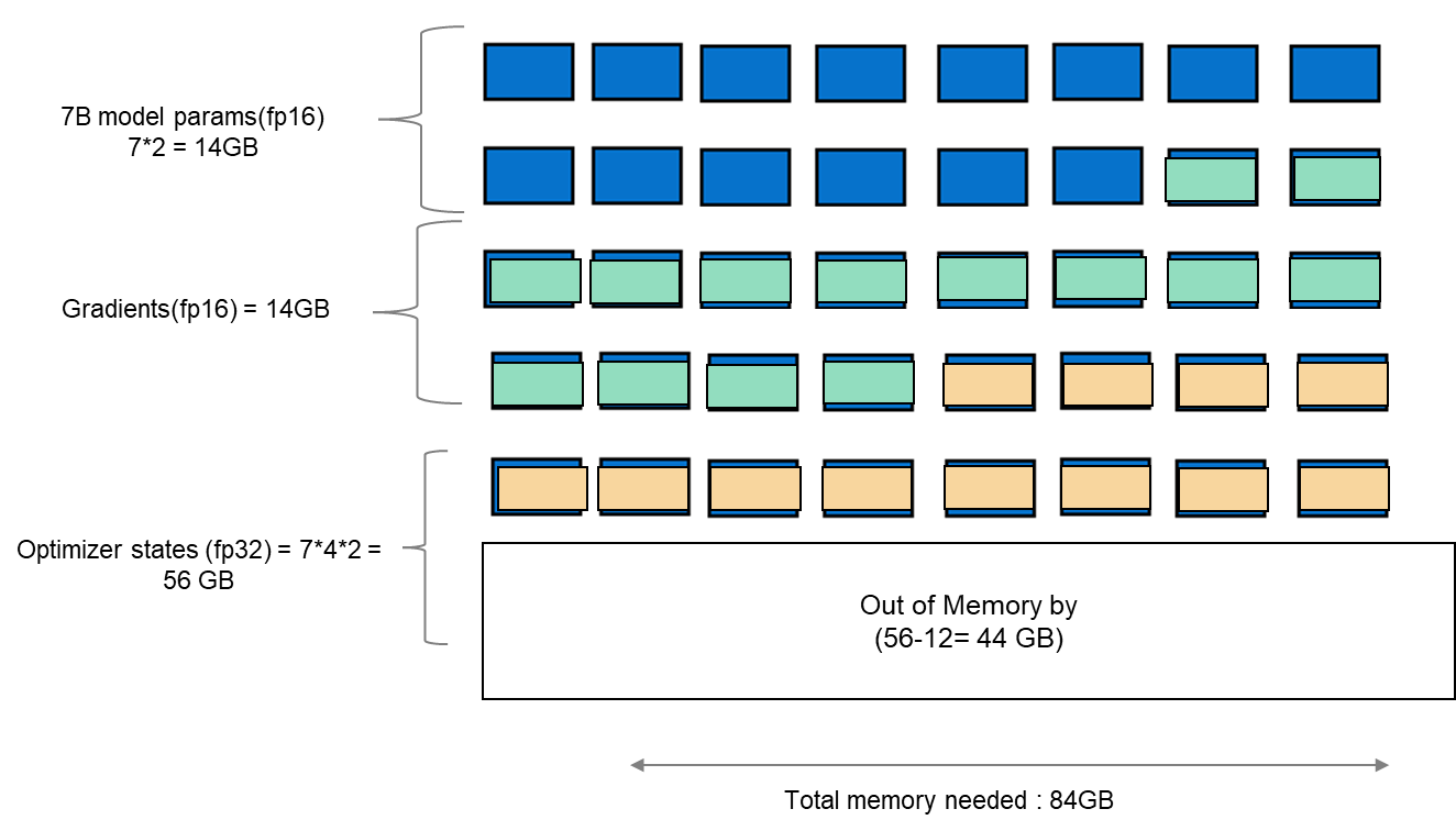
Figure 1. Schematic showing memory footprint of standard fine-tuning with Llama 27B model.

Fine-tuning method

LoRA is an efficient fine-tuning method where instead of finetuning all the weights that constitute the weight matrix of the pre-trained LLM, it optimizes rank decomposition matrices of the dense layers to change during adaptation. These matrices constitute the LoRA adapter. This fine-tuned adapter is then merged with the pre-trained model and used for inferencing. The number of parameters is determined by the rank and shape of the original weights. In practice, trainable parameters vary as low as 0.1% to 1% of all the parameters. As the number of parameters needing fine-tuning decreases, the size of gradients and optimizer states attached to them decrease accordingly. Thus, the overall size of the loaded model reduces. For example, the Llama 2 7B model parameters could be loaded in int8 (1 byte), with 1 GB trainable parameters loaded in fp16 (2 bytes). Hence, the size of the gradient (fp16), optimizer states (fp32), and activations (fp32) aggregates to approximately 7-9 GB. This brings the total size of the loaded model to be fine-tuned to 15-17 GB, as illustrated in figure 2.

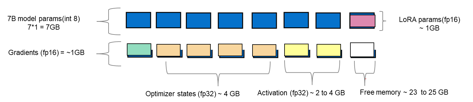
Figure 2. Schematic showing an example of memory footprint of LoRA fine tuning with Llama 2 7B model.

Experimental setup 

A model characterization gives readers valuable insight into GPU memory utilization, training loss, and computational efficiency measured during fine-tuning by varying the batch size and observing out-of-memory (OOM) occurrence for a given dataset. In table 1, we show resource profiling when fine-tuning Llama 2 7B-chat model using LoRA technique on PowerEdge R760xa with 1*A100-40 GB on Open- source SAMsum dataset. To measure tera floating-point operations (TFLOPs) on the GPU, the DeepSpeed Flops Profiler was used. Table 1 gives the detail on the system used for this experiment.

Table 1. Actual memory footprint of Llama 27B model using LoRA technique in our experiment.

System configuration

In this section, we list the hardware and software system configuration of the R760xa PowerEdge server used in this experiment for the fine-tuning work of Llama-2 7B model.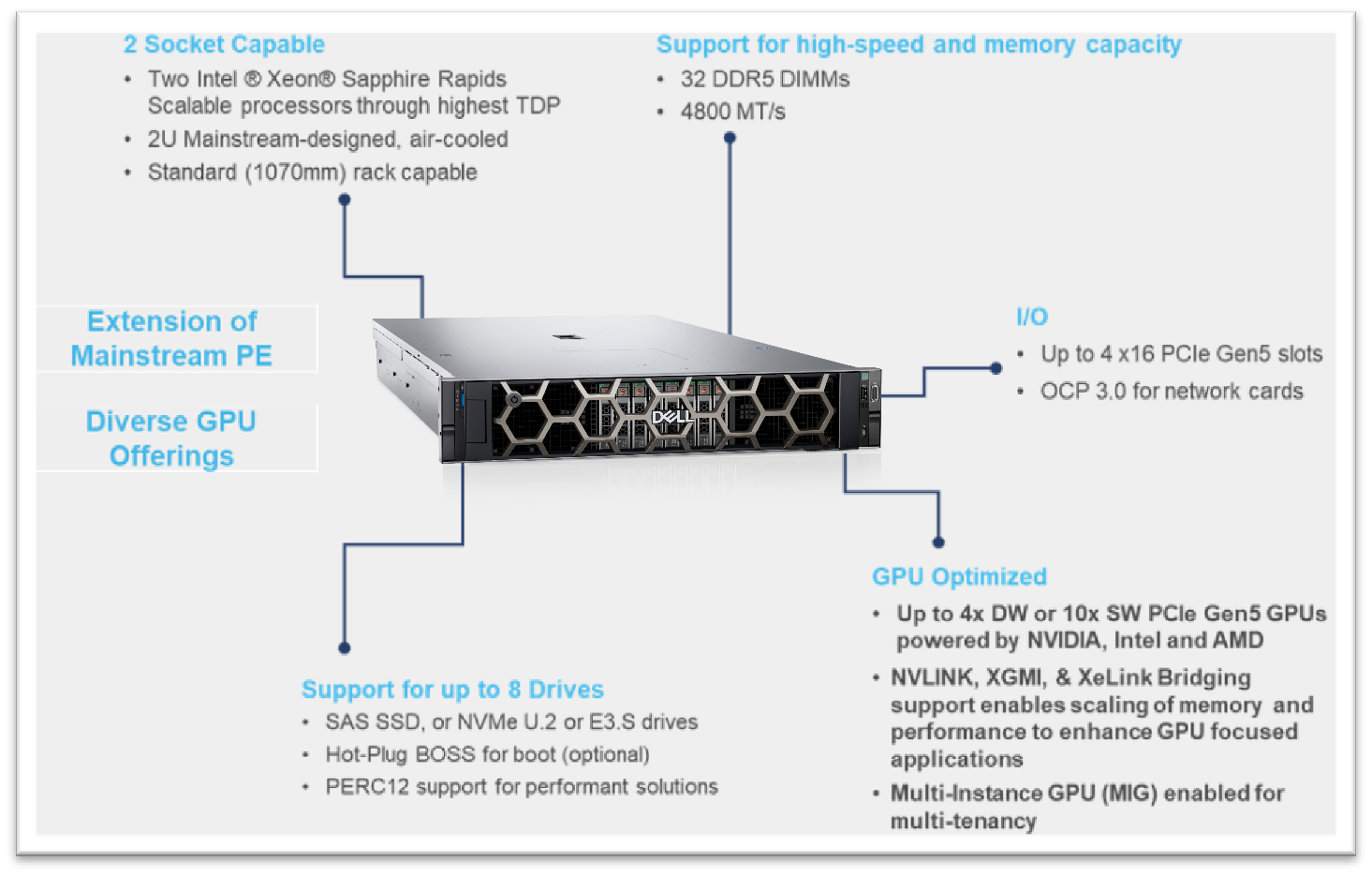

Figure 3. R760XA Specs

Table 2. Hardware and software configuration of the system 

Dataset

The SAMsum dataset – size 2.94 MB – consists of approximately 16,000 rows (Train, Test, and Validation) of English dialogues and their summary. This data was used to fine-tune the Llama 2 7B model. We preprocess this data in the format of a prompt to be fed to the model for fine-tuning. In the JSON format, prompts and responses were used to train the model. During this process, PyTorch batches the data (about 10 to 11 rows per batch) and concatenates them. Thus, a total of 1,555 batches are created by preprocessing the training split of the dataset. These batches are then passed to the model in chunks for fine-tuning.

Fine-tuning steps

1. Download the Llama 2 model
   • The model is available either from Meta’s git repository or Hugging Face, however to access the model, you will need to submit the required registration form for Meta AI license agreement 
   • The details can be found in our previous work here
2. Convert the model from the Meta’s git repo to a Hugging face model type in order to use the PEFT libraries used in the LoRA technique
   • Use the following commands to convert the model 

     ## Install HuggingFace Transformers from source pip freeze | grep transformers ## verify it is version 4.31.0 or higher   git clone git@github.com:huggingface/transformers.git cd transformers pip install protobuf python src/transformers/models/llama/convert_llama_weights_to_hf.py \    --input_dir /path/to/downloaded/llama/weights --model_size 7B --output_dir /output/path

3. Build a conda environment and then git clone the example fine-tuning recipes from Meta’s git repository to get started
   • We have modified the code base to include Deepspeed flops profiler and nvitop to profile the GPU
4. Load the dataset using the dataloader library of hugging face and, if need be, perform preprocessing
5. Input the config file entries with respect to PEFT methods, model name, output directory, save model location, etc 
   • The following is the example code snippet

 train_config:

    model_name: str="path_of_base_hugging_face_llama_model"    

    run_validation: bool=True

    batch_size_training: int=7

    num_epochs: int=1  

    val_batch_size: int=1

    dataset = "dataset_name" 

    peft_method: str = "lora"

    output_dir: str = "path_to_save_fine_tuning_model"
    save_model: bool = True

 6. Run the following command to perform fine tuning on a single GPU

python3 llama_finetuning.py  --use_peft --peft_method lora --quantization --model_name location_of_hugging_face_model

Figure 4 shows fine tuning with LoRA technique on 1*A100 (40GiB) with Batch size = 7 on SAMsum dataset, which took 83 mins to complete.

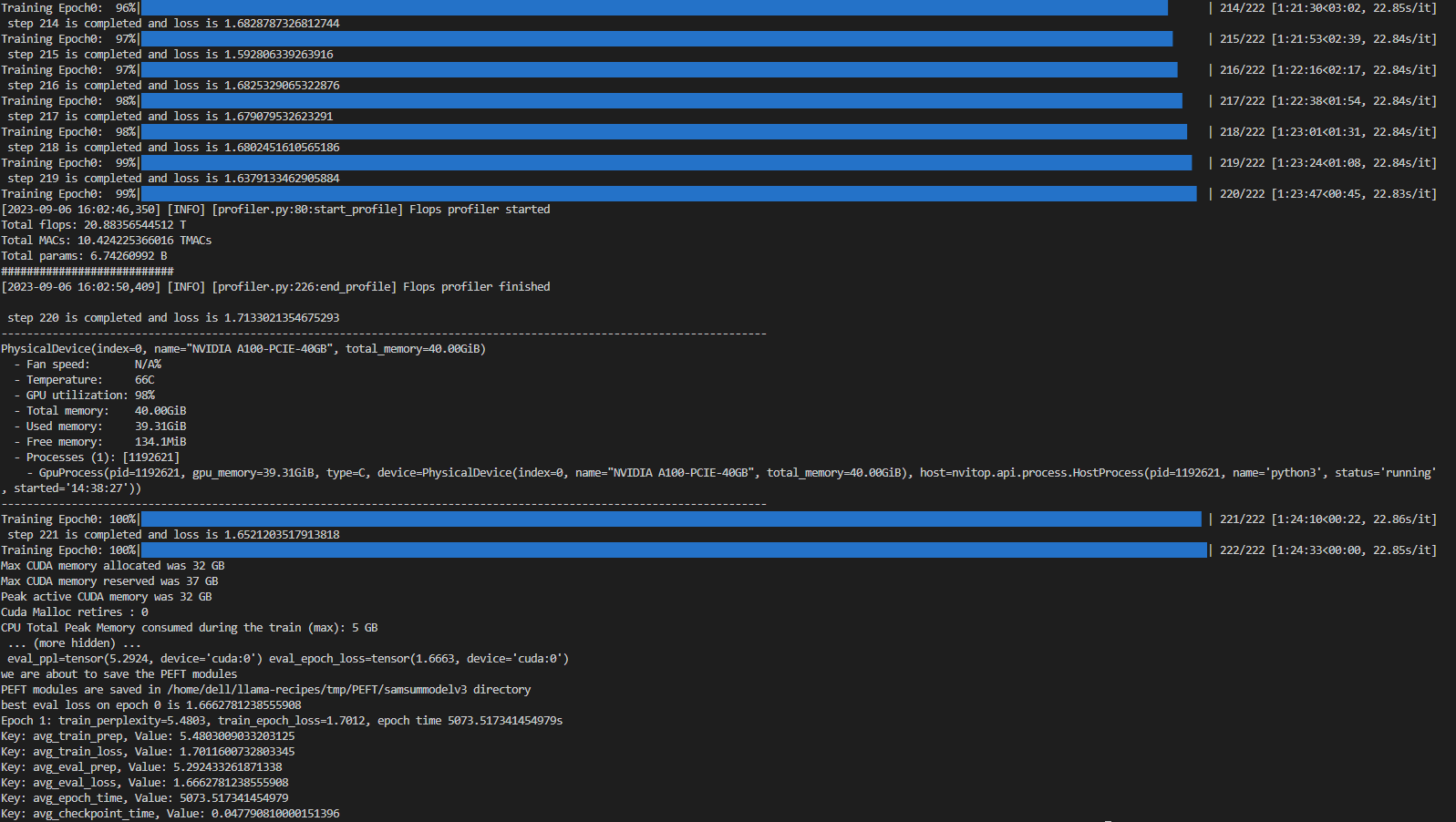
Figure 4. Example screenshot of fine-tuning with LoRA on SAMsum dataset

Experiment results

The fine-tuning experiments were run at batch sizes 4 and 7. For these two scenarios, we calculated training losses, GPU utilization, and GPU throughput. We found that at batch size 8, we encountered an out-of-memory (OOM) error for the given dataset on 1*A100 with 40 GB. 

When a dialogue was sent to the base 7B model, the summarization results are not proper as shown in figure 5. After fine-tuning the base model on the SAMsum dataset, the same dialogue prompts a proper summarized result as shown in figure 6. The difference in results shows that fine-tuning succeeded. 

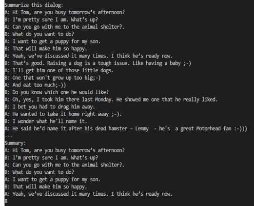
Figure 5. Summarization results from the base model.

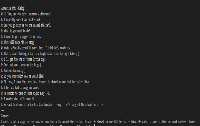
Figure 6. Summarization results from the fine-tuned model.

Figures 7 and 8 show the training losses at batch size 4 and 7 respectively. We found that even after increasing the batch size by approximately 2x times, the model training performance did not degrade. 

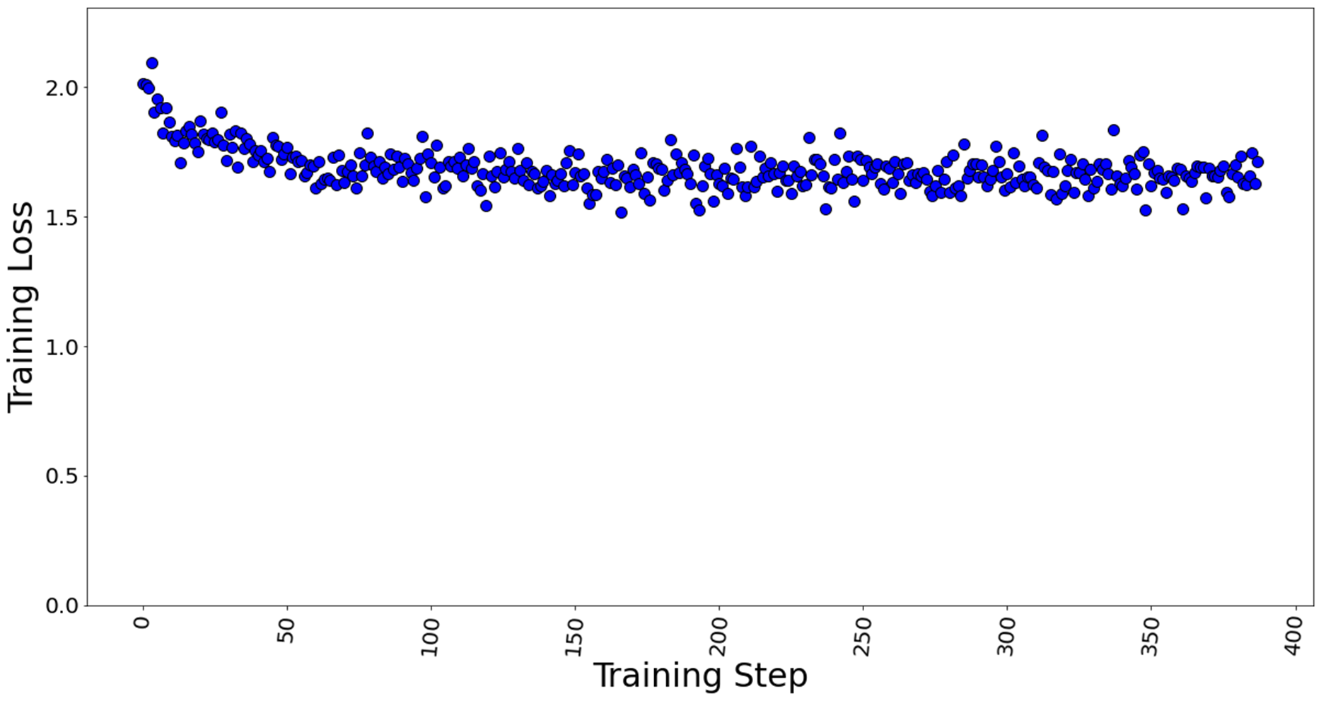
Figure 7. Training loss with batch size = 4, a total of 388 training steps in 1 epoch.

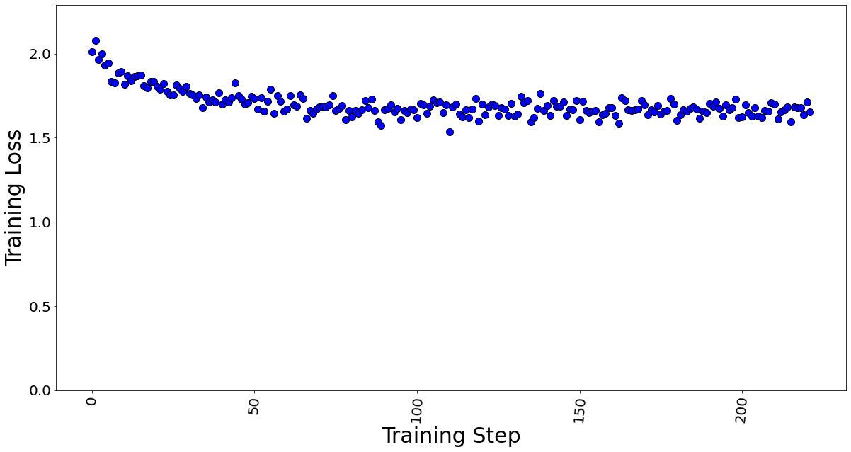
Figure 8. Training loss with batch size = 7, a total of 222 training steps in 1 epoch.

The GPU memory utilization was captured with LoRA technique in Table 3. At batch size 1, used memory was 9.31 GB. At batch size of 4, used memory was 26.21 GB. At batch size 7, memory used was 39.31 GB. Going further, we see an OOM at batch size 8 for 40 GB GPU card. The memory usage remains constant throughout fine-tuning, as shown in Figure 9, and is dependent on the batch size. We calculated the reserved memory per batch to be 4.302 GB on 1*A100. 

Table 3. The GPU memory utilization is captured by varying the max. batch size parameter.

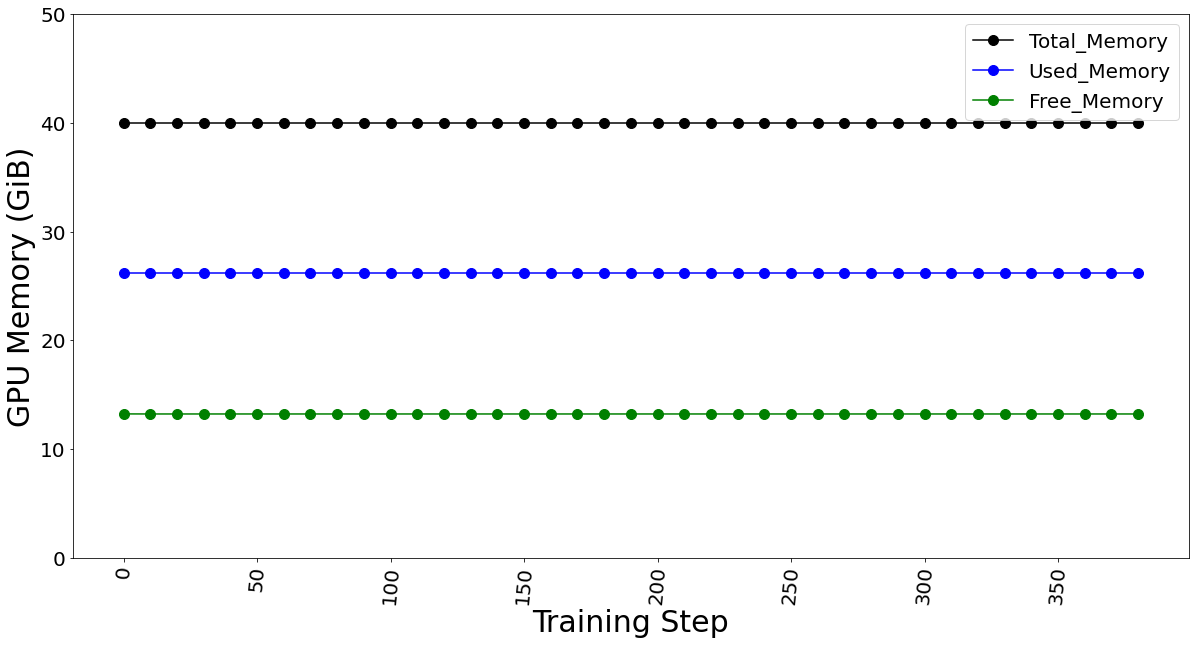
Figure 9. GPU memory utilization for batch size 4 (which remains constant for fine-tuning)

The GPU TFLOP was determined using DeepSpeed Profiler, and we found that FLOPs vary linearly with the number of batches sent in each step, indicating that FLOPs per token is the constant.

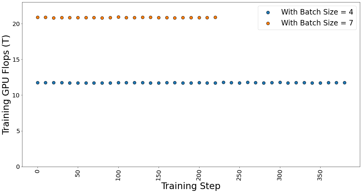
Figure 10. Training GPU TFlops for batch sizes 4 and 7 while fine-tuning the model.

The GPU multiple-accumulate operations (MACs), which are common operations performed in deep learning models, are also determined. We found that MACs also follow a linear dependency on the batch size and hence constant per token. 

Figure 11. GPU MACs for batch sizes 4 and 7 while the fine-tuning the model. 

The time taken for fine-tuning, which is also known as epoch time, is given in table 4. It shows that the training time does not vary much, which strengthens our argument that the FLOPs per token is constant. Hence, the total training time is independent of the batch size.

Table 4. Data showing the time taken by the fine-tuning process.

Conclusion and Recommendation

1. We show that using a PEFT technique like LoRA can help reduce the memory requirement for fine-tuning a large-language model on a proprietary dataset. In our case, we use a Dell PowerEdge R760xa featuring the NVIDIA A100-40GB GPU to fine-tune a Llama 2 7B model.
2. We recommend using a lower batch size to minimize automatic memory allocation, which could be utilized in the case of a larger dataset. We have shown that a lower batch size affects neither the training time nor training performance.  
3. The memory capacity required to fine-tune the Llama 2 7B model was reduced from 84GB to a level that easily fits on the 1*A100 40 GB card by using the LoRA technique. 

Resources

• Llama 2: Inferencing on a Single GPU
• LoRA: Low-Rank Adaptation of Large Language Models
• Hugging Face Samsum Dataset

Author: Khushboo Rathi khushboo_rathi@dell.com | www.linkedin.com/in/khushboorathi

Co-author: Bhavesh Patel bhavesh_a_patel@dell.com | www.linkedin.com/in/BPat