
Assets

Introduction to Using the GenAI-Perf Tool on Dell Servers


Mon, 22 Jul 2024 13:16:51 -0000
|Read Time: 0 minutes
Overview
Performance analysis is a critical component that ensures the efficiency and reliability of models during the inference phase of a machine learning life cycle. For example, using a concurrency mode or request rate mode to simulate load on a server helps you understand various load conditions that are crucial for capacity planning and resource allocation. Depending on the use case, the analysis helps to replicate real-world scenarios. It can optimize performance to maintain a specific concurrency of incoming requests to the server, ensuring that the server can handle constant load or bursty traffic patterns. Providing a comprehensive view of the models’ performance enables data scientists to build models that are not only accurate but also robust and efficient.
Triton Performance Analyzer is a CLI tool that analyzes and optimizes the performance of Triton-based systems. It provides detailed information about the systems’ performance, including metrics related to GPU, CPU, and memory. It can also collect custom metrics using Triton’s C API. The tool supports various inference load modes and performance measurement modes.
The Triton Performance Analyzer can help identify performance bottlenecks, optimize system performance, troubleshoot issues, and more. In the suite of Tritons’ performance analysis tools, GenAI-Perf (which was released recently) uses Perf Analyzer in the backend. The GenAI-Perf tool can be used to gather various LLM metrics.
This blog focuses on the capabilities and use of GenAI-Perf.
GenAI-Perf
GenAI-Perf is a command-line performance measurement tool that is customized to collect metrics that are more useful when analyzing an LLM’s performance. These metrics include, output token throughput, time to first token, inter-token latency, and request throughput.
The metrics can:
- Analyze the system performance
- Determine how quickly the system starts processing the request
- Provide the overall time taken by the system to completely process a request
- Retrieve a granular view of how fast the system can generate individual parts of the response
- Provide a general view on the system’s efficiency in generating tokens
This blog also describes how to collect these metrics and automatically create plots using GenAI-Perf.
Implementation
The following steps guide you through the process of using GenAI-Perf. In this example, we collect metrics from a Llama 3 model.
Triton Inference Server
Before running the GenAI-Perf tool, launch Triton Inference Server with your Large Language Model (LLM) of choice.
The following procedure starts Llama 3 70 B and runs on Triton Inference Server v24.05. For more information about how to convert HuggingFace weights to run on Triton Inference Server, see the Converting Hugging Face Large Language Models to TensorRT-LLM blog.
The following example shows a sample command to start a Triton container:
docker run --rm -it --net host --shm-size=128g \
--ulimit memlock=-1 --ulimit stack=67108864 --gpus all \
-v $(pwd)/llama3-70b-instruct-ifb:/llama_ifb \
-v $(pwd)/scripts:/opt/scripts \
nvcr.io/nvidia/tritonserver:24.05-trtllm-python-py3
Because Llama 3 is a gated model distributed by Hugging Face, you must request access to Llama 3 using Hugging Face and then create a token. For more information about Hugging Face tokens, see https://huggingface.co/docs/text-generation-inference/en/basic_tutorials/gated_model_access.
An easy method to use your token with Triton is to log in to Hugging Face, which caches a local token:
huggingface-cli login --token hf_Enter_Your_Token
The following example shows a sample command to start the inference:
python3 /opt/scripts/launch_triton_server.py --model_repo /llama_ifb/ --world_size 4
NIM for LLMs
Another method to deploy the Llama 3 model is to use the NVIDIA Inference Microservices (NIM). For more information about how to deploy NIM on the Dell PowerEdge XE9680 server, see Introduction to NVIDIA Inference Microservices, aka NIM. Also, see NVIDIA NIM for LLMs - Introduction.
The following example shows a sample script to start NIM with Llama 3 70b Instruct:
export NGC_API_KEY=<enter-your-key>
export CONTAINER_NAME=meta-llama3-70b-instruct
export IMG_NAME="nvcr.io/nim/meta/llama3-70b-instruct:1.0.0"
export LOCAL_NIM_CACHE=/aipsf810/project-helix/NIM/nim
mkdir -p "$LOCAL_NIM_CACHE"
docker run -it --rm --name=$CONTAINER_NAME \
--runtime=nvidia \
--gpus all \
--shm-size=16GB \
-e NGC_API_KEY \
-v "$LOCAL_NIM_CACHE:/opt/nim/.cache" \
-u $(id -u) \
-p 8000:8000 \
$IMG_NAME
Triton SDK container
After the Triton Inference container is launched and the inference is started, run the Triton Server SDK:
docker run -it --net=host --gpus=all \
nvcr.io/nvidia/tritonserver:24.05-py3-sdk
You can install the GenAI-Perf tool using pip. In our example, we use the NGC container, which is easier to use and manage.
Measure throughput and latency
When the containers are running, log in to the SDK container and run the GenAI-Perf tool.
The following example shows a sample command:
genai-perf \
-m ensemble \
--service-kind triton \
--backend tensorrtllm \
--num-prompts 100 \
--random-seed 123 \
--synthetic-input-tokens-mean 200 \
--synthetic-input-tokens-stddev 0 \
--streaming \
--output-tokens-mean 100 \
--output-tokens-stddev 0 \
--output-tokens-mean-deterministic \
--tokenizer hf-internal-testing/llama-tokenizer \
--concurrency 1 \
--generate-plots \
--measurement-interval 10000 \
--profile-export-file profile_export.json \
--url localhost:8001
This command produces values similar to the values in the following table:
| Statistic | Average | Minimum | Maximum | p99 | p90 | p75 |
| Time to first token (ns) Inter token latency (ns) Request latency (ns) Number of output tokens Number of input tokens | 40,375,620 17,272,993 1,815,146,838 108 200 | 37,453,094 5,665,738 1,811,433,087 100 200 | 74,652,113 19,084,237 1,850,664,440 123 200 | 69,046,198 19,024,802 1,844,310,335 122 200 | 39,642,518 18,060,240 1,814,057,039 116 200 | 38,639,988 18,023,915 1,813,603,920 112 200 |
Output token throughput (per sec): 59.63
Request throughput (per sec): 0.55
See Metrics at https://docs.nvidia.com/deeplearning/triton-inference-server/user-guide/docs/client/src/c%2B%2B/perf_analyzer/genai-perf/README.html#metrics for more information.
To run the performance tool with NIM, you must change parameters such as the model name, service-kind, endpoint-type, and so on, as shown in the following example:
genai-perf \
-m meta/llama3-70b-instruct \
--service-kind openai \
--endpoint-type chat \
--backend tensorrtllm \
--num-prompts 100 \
--random-seed 123 \
--synthetic-input-tokens-mean 200 \
--synthetic-input-tokens-stddev 0 \
--streaming \
--output-tokens-mean 100 \
--output-tokens-stddev 0 \
--tokenizer hf-internal-testing/llama-tokenizer \
--concurrency 1 \
--measurement-interval 10000 \
--profile-export-file profile_export.json \
--url localhost:8000
Results
The GenAI-Perf tool saves the output to the artifacts directory by default. Each run creates an artifacts/<model-name>_<service-kind>_<backend>_<concurrency"X"> directory.
The following example shows a sample directory:
ll artifacts/ensemble-triton-tensorrtllm-concurrency1/
total 2800
drwxr-xr-x  3 user user     127 Jun 10 13:40 ./
drwxr-xr-x 10 user user    4096 Jun 10 13:34 ../
-rw-r--r--  1 user user   16942 Jun 10 13:40 all_data.gzip
-rw-r--r--  1 user user  126845 Jun 10 13:40 llm_inputs.json
drwxr-xr-x  2 user user    4096 Jun 10 12:24 plots/
-rw-r--r--  1 user user 2703714 Jun 10 13:40 profile_export.json
-rw-r--r--  1 user user     577 Jun 10 13:40 profile_export_genai_perf.csv
The profile_export_genai_perf.csv file provides the same results that are displayed during the test.
You can also plot charts that are based on the data automatically. To enable this feature, include --generate-plots in the command.
The following figure shows the distribution of input tokens to generated tokens. This metric is useful to understand how the model responds to different lengths of input.
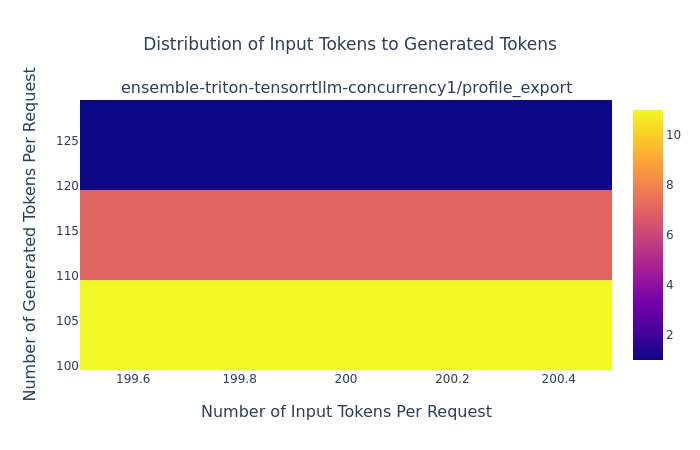
Figure 1: Distribution of input tokens to generated tokens
The following figure shows a scatter plot of how token-to-token latency varies with output token position. These results show how quickly tokens are generated and how consistent the generation is regarding various output token positions.
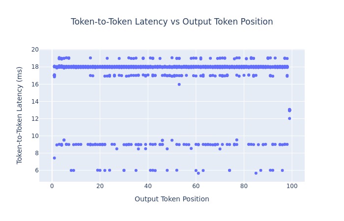
Figure 2: Token-to-token latency compared to output token position
Conclusion
Performance analysis during the inference phase is crucial as it directly impacts the overall effectiveness of a machine learning solution. Tools such as GenAI-Perf provide comprehensive information that help anyone looking to deploy optimized LLMs in production. The NVIDIA Triton suite has been extensively tested on Dell servers and can be used to capture important LLM metrics with minimum effort. The GenAI-Perf tool is easy to use and produces extensive data that can be used to tune your LLM for optimal performance.

Scaling Deep Learning Workloads in a GPU Accelerated Virtualized Environment
Mon, 29 Apr 2024 14:30:31 -0000
|Read Time: 0 minutes
Introduction
Demand for compute, parallel, and distributed training is ever increasing in the field of deep learning (DL). The introduction of large-scale language models such as Megatron-Turing NLG (530 billion parameters; see References 1 below) highlights the need for newer techniques to handle parallelism in large-scale model training. Impressive results from transformer models in natural language have paved a way for researchers to apply transformer-based models in computer vision. The ViT-Huge (632 million parameters; see References 2 below) model, which uses a pure transformer applied to image patches, achieves amazing results in image classification tasks compared to state-of-the-art convolutional neural networks.
Larger DL models require more training time to achieve convergence. Even smaller models such as EfficientNet (43 million parameters; see References 3 below) and EfficientNetV2 (24 million parameters; see References 3 below) can take several days to train depending on the size of data and the compute used. These results clearly show the need to train models across multiple compute nodes with GPUs to reduce the training time. Data scientists and machine learning engineers can benefit by distributing the training of a DL model across multiple nodes. The Dell Validated Design for AI shows how software-defined infrastructure with virtualized GPUs is highly performant and suitable for AI (Artificial Intelligence) workloads. Different AI workloads require different resources sizing, isolation of resources, use of GPUs, and a better way to scale across multiple nodes to handle the compute-intensive DL workloads.
This blog demonstrates the use and performance across various settings such as multinode and multi-GPU workloads on Dell PowerEdge servers with NVIDIA GPUs and VMware vSphere.
System Details
The following table provides the system details:
Table 1: System details
Component | Details |
Server | Dell PowerEdge R750xa (NVIDIA-Certified System) |
Processor | 2 x Intel Xeon Gold 6338 CPU @ 2.00 GHz |
GPU | 4 x NVIDIA A100 PCIe |
Network Adapter | Mellanox ConnectX-6 Dual port 100 GbE |
Storage | Dell PowerScale |
ESXi Version | 7.0.3 |
BIOS Version | 1.1.3 |
GPU Driver Version | 470.82.01 |
CUDA Version | 11.4 |
Setup for multinode experiments
To achieve the best performance for distributed training, we need to perform the following high-level steps when the ESXi server and virtual machines (VMs) are created:
- Enable Address Translation Services (ATS) on VMware ESXi and VMs to enable peer to peer (P2P) transfers with high performance.
- Enable ATS on the ConnectX-6 NIC.
- Use the ibdev2netdev utility to display the installed Mellanox ConnectX-6 card and mapping between logical and physical ports, and enable the required ports.
- Create a Docker container with Mellanox OFED drivers, Open MPI Library, and NVIDIA optimized TensorFlow (the DL framework that is used in the following performance tests).
- Set up a keyless SSH login between VMs.
- When configuring multiple GPUs in the VM, connect the GPUs with NVLINK.
Performance evaluation
For the evaluation, we used VMs with 32 CPUs, 64 GB of memory, and GPUs (depending on the experiment). The evaluation of the training performance (throughput) is based on the following scenarios:
- Scenario 1—Single node with multiple VMs and multi-GPU model training
- Scenario 2—Multinode model training (distributed training)
Scenario 1
Imagine the case in which there are multiple data scientists working on building and training different models. It is vital to strictly isolate resources that are shared between the data scientists to run their respective experiments. How effectively can the data scientists use the resources available?
The following figure shows several experiments on a single node with four GPUs and the performance results. For each of these experiments, we run tf_cnn_benchmarks with the ResNet50 model with a batch size of 1024 using synthetic data.
Note: The NVIDIA A100 GPU supports a NVLink bridge connection with a single adjacent NVIDIA A100 GPU. Therefore, the maximum number of GPUs added to a single VM for multi-GPU experiments on a Dell PowerEdge R750xa server is two.
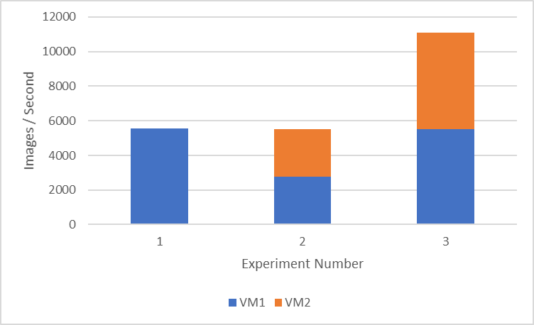
Figure 1: Performance comparison of multi-VMs and multi-GPUs on a single node
Figure 1 shows the throughput (the average on three runs) of three different experiment setups:
- Setup 1 consists of a single VM with two GPUs. This setup might be beneficial to run a machine learning workload, which needs more GPUs for faster training (5500 images/second) but still allows the remaining resources in the available node for other data scientists to use.
- Setup 2 consists of two VMs with one GPU each. We get approximately 2700 images/second on each VM, which can be useful to run multiple hyper-parameter search experiments to fine-tune the model.
- Setup 3 consists of two VMs with two GPUs each. We use all the GPUs available in the node and show the maximum cumulative throughput of approximately 11000 images/second between two VMs.
Scenario 2
Training large DL models requires a large amount of compute. We also need to ensure that the training is completed in an acceptable amount of time. Efficient parallelization of deep neural networks across multiple servers is important to achieve this requirement. There are two main algorithms when we address distributed training, data parallelism, and model parallelism. Data parallelism allows the same model to be replicated in all nodes, and we feed different batches of input data to each node. In model parallelism, we divide the model weights to each node and the same minibatch data is trained across the nodes.
In this scenario, we look at the performance of data parallelism while training the model using multiple nodes. Each node receives different minibatch data. In our experiments, we scale to four nodes with one VM and one GPU each.
To help with scaling models to multiple nodes, we use Horovod (see References 6 below ), which is a distributed DL training framework. Horovod uses the Message Passing Interface (MPI) to effectively communicate between the processes.
MPI concepts include:
- Size indicates the total number of processes. In our case, the size is four processes.
- Rank is the unique ID for each process.
- Local rank indicates the unique process ID in a node. In our case, there is only one GPU in each node.
- The Allreduce operation aggregates data among multiple processes and redistributes them back to the process.
- The Allgather operation is used to gather data from all the processes.
- The Broadcast operation is used to broadcast data from one process identified by root to other processes.
The following table provides the scaling experiment results:
Table 2: Scaling experiments results
Number of nodes | VM Throughput (images/second) |
1 | 2757.21 |
2 | 5391.751667 |
4 | 10675.0925 |
For the scaling experiment results in the table, we run tf_cnn_benchmarks with the ResNet50 model with a batch size of 1024 using synthetic data. This experiment is a weak scaling-based experiment; therefore, the same local batch size of 1024 is used as we scale across nodes.
The following figure shows the plot of speedup analysis of scaling experiment:
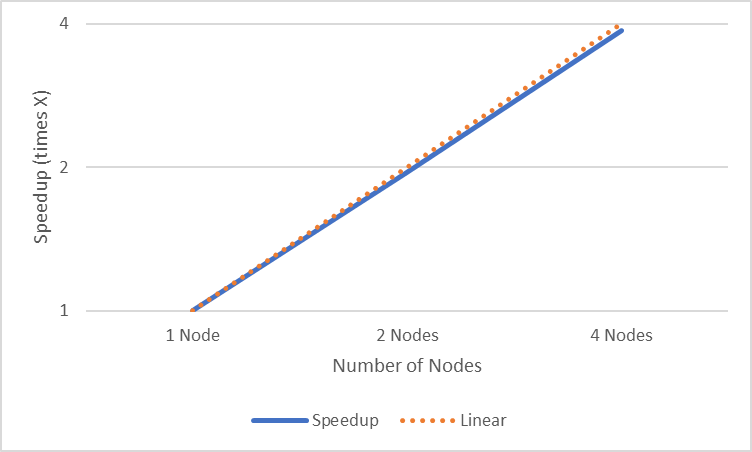
Figure 2: Speedup analysis of scaling experiment
The speedup analysis in Figure 2 shows the speedup (times X) when scaling up to four nodes. We can clearly see that it is almost linear scaling as we increase the number of nodes.
The following figure shows how multinode distributed training on VMs compares to running the same experiments on bare metal (BM) servers:
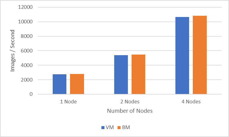
Figure 3: Performance comparison between VMs and BM servers
The four-nodes experiment (one GPU per node) achieves a throughput of 10675 images/second in the VM environment while the similarly configured BM run achieves a throughput of 10818 images/second. One-, two-, and four-node experiments show a percentage difference of less than two percent between BM experiments and VM experiments.
Conclusion
In this blog, we described how to set up the ESXi server and VMs to be able to run multinode experiments. We examined various scenarios in which data scientists can benefit from multi-GPU experiments and their corresponding performance. The multinode scaling experiments showed how the speedup is closer to linear scaling. We also examined how VM-based distributed training compares to BM-server based distributed training. In upcoming blogs, we will look at best practices for multinode vGPU training, and the use and performance of NVIDIA Multi-Instance GPU (MIG) for various deep learning workloads.
References
- Using DeepSpeed and Megatron to Train Megatron-Turing NLG 530B, the World’s Largest and Most Powerful Generative Language Model
- An Image is Worth 16x16 Words: Transformers for Image Recognition at Scale
- EfficientNetV2: Smaller Models and Faster Training
- Virtualizing GPUs for AI with VMware and NVIDIA Based on Dell Infrastructure Design Guide
- https://github.com/horovod/horovod
Contributors
Contributors to this blog: Prem Pradeep Motgi and Sarvani Vemulapalli

Effectiveness of Large Batch Training for Neural Machine Translation with Intel Xeon
Wed, 24 Apr 2024 15:17:12 -0000
|Read Time: 0 minutes
We know that using really large batch sizes during training can cause models to poorly generalize. But how do large batches actually affect the generalization and optimization of neural network models? 2018 was a great year for research on Neural Machine Translation (NMT). We’ve seen an explosion in the number of research papers published in this field, ranging from descriptions of new and interesting architectures to efficient training techniques. Research papers have shown how larger batch sizes and reduced precision can help to improve both the training time and quality.
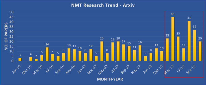
Figure 1: Numbers of papers published in Arxiv with ‘neural machine translation’ in the title or abstract in the ‘cs’ category.
In our previous blogs, we showed how to effectively scale an NMT system, as well as some of the challenges associated with scaling. In this blog, we will explore the effectiveness of large batch training using Intel® Xeon® Scalable processors. The work discussed in the blog is based on neural network training performed using Zenith supercomputer at Dell EMC’s HPC and AI Innovation Lab.
System Information
CPU Model | Intel® Xeon® Gold 6148 CPU @ 2.40GHz |
Operating System | Red Hat Enterprise Linux Server release 7.4 (Maipo) |
Tensorflow Version | Anaconda TensorFlow 1.12.0 with Intel® MKL |
Horovod Version | 0.15.2 |
MPI | MVAPICH2 2.1 |
Incredible strong scaling efficiency helps to dramatically reduce the time to solution of the model. To best visualize this, consider figure 2. The time to solution drops from around 1 month on a single node to just over 6 hours using 200 nodes. This 121x faster solution would significantly help the productivity of NMT researchers using CPU-based HPC infrastructures. The results observed were based on the models achieving a baseline BLEU score (case-sensitive) of 27.5.
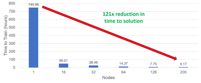
Figure 2: Time to train the model to solution
For the single node case, we have used the largest batch size that could fit in a node's memory, 25,600 tokens per worker. For all other cases, we use a global batch size of 819,200, leading to per-worker batch sizes of 25,600 in the 16-node case, down to only 2,048 in the 200-node case. The number of training iterations is similar for all experiments in the 16-200 node range and is increased by a factor of 16 for the single-node case (to compensate for the larger batch).
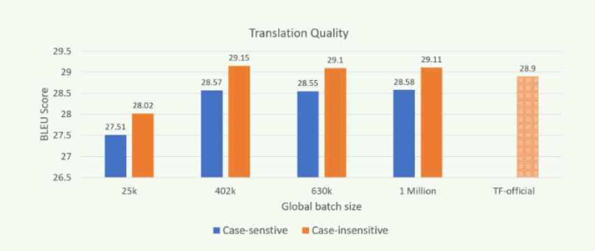
Figure 3: Translation quality (BLEU) when trained with different batch sizes on Zenith.
Scaling out the “transformer” model training using MPI and Horovod improves throughput performance while producing models of similar translation quality as shown in Figure 3. The results were obtained by using newstest2014 as the test set. Models of comparable quality can be trained in a reduced amount of time by scaling computation over many more nodes, and with larger global batch sizes (GBZ). Our experiments on Zenith demonstrate the ability to train models of comparable or higher translation quality (as measured by BLEU score) than the reported best for TensorFlow's official model, even when training with batches of a million or more tokens.
Note: The results shown in figure 3 were obtained by using the settings mentioned in our previous blog and by using Open MPI.
Conclusion
Here in this blog, we showed the generalization of large batch training of NMT model. We also showed how efficiently Intel® Xeon® Scalable processors are able to scale and reduce the time to solution. We hope this would benefit the productivity of the NMT research community using CPU-based HPC infrastructures.
Srinivas Varadharajan - Machine Learning/Deep Learning Developer
Twitter: @sedentary_yoda
LinkedIn: https://www.linkedin.com/in/srinivasvaradharajan

Scaling Neural Machine Translation - Challenges and Solution
Wed, 24 Apr 2024 15:15:31 -0000
|Read Time: 0 minutes
As I mentioned in our previous blog post, the translation quality of neural machine translation (NMT) systems has improved immensely in recent years. However, these models still take considerable time to train, and little work has been focused on improving their time to solution. Distributed training across multiple compute nodes can potentially improve the time to train, but there are various challenges associated with scale-out training of NMT systems.
In this blog, we highlight solutions developed at Dell EMC which address a few common issues encountered when scaling an NMT architecture like the Transformer model in TensorFlow, highlight the performance benefits associated with these solutions. All of the experiments and results obtained used Zenith, DellEMC’s very own Intel® Xeon® Scalable processor-based supercomputer, which is housed in the Dell EMC HPC & AI Innovation Lab in Austin, Texas.
Performance degradation and OOM errors
One of the main roadblocks to scaling NMT models is the memory required to accumulate gradients. When training neural networks, the gradients are vectors – or directional arrays – of numbers that roughly correspond to the difference between the current network weights and a set of weights that provide a better solution. Essentially, the gradients point each weight value in a different, and hopefully, a better direction which leads to better solutions. While convolutional neural networks for image classification use dense gradient vectors which can be easily worked with, the design of the transformer model uses an embedding layer that does not necessarily scale well to multiple servers.
This design causes severe performance degradation and out of memory (OOM) errors because TensorFlow does not accumulate the embedding layer gradients correctly. Gradients from the embedding layer are sparse, whereas the gradients from the projection matrix are dense. TensorFlow then accumulates both of these tensors as sparse objects. This has a dramatic effect on TensorFlow’s gradient accumulation strategy, and subsequently on the total size of the accumulated gradient tensor. This results in large message buffers which scale linearly with the number of processes, thereby causing segmentation faults or out-of-memory errors.
The assumed-sparse tensors make Horovod (the distributed training framework used with TensorFlow) to perform gradient accumulation by MPI_Gather rather than MPI_Reduce. To fix this issue, we can convert all assumed sparse tensors to dense tensors. This is done by adding the flag “sparse_as_dense=True” in Horovod’s DistributedOptimizer method.
opt = hvd.DistributedOptimizer(opt, sparse_as_dense=True)
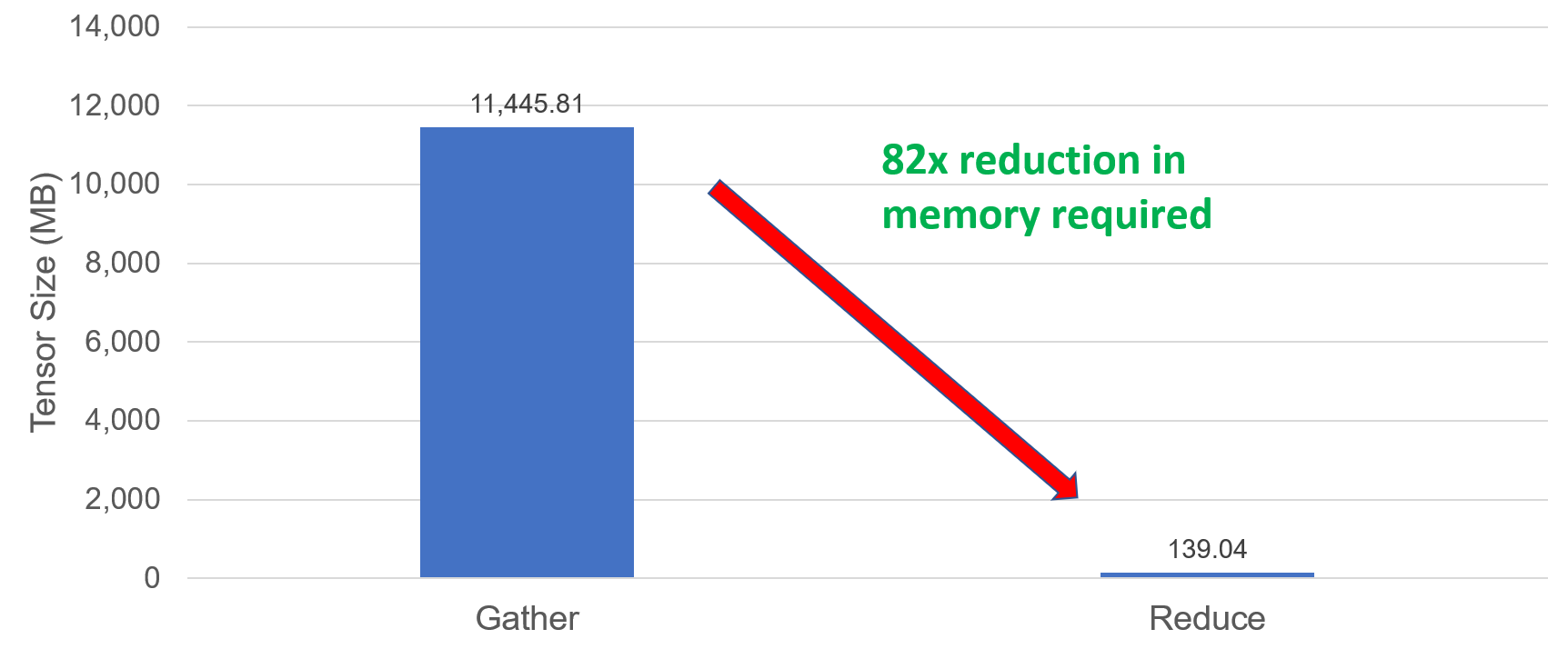
Figure 1: Accumulate size
Figure 1 shows the accumulation size when using 64 nodes (1ppn, batch_size=5000 tokens). There’s an 82x reduction in accumulation size when the assumed sparse tensors are converted to dense. This solution allows to scale and train the model using 100’s of nodes.
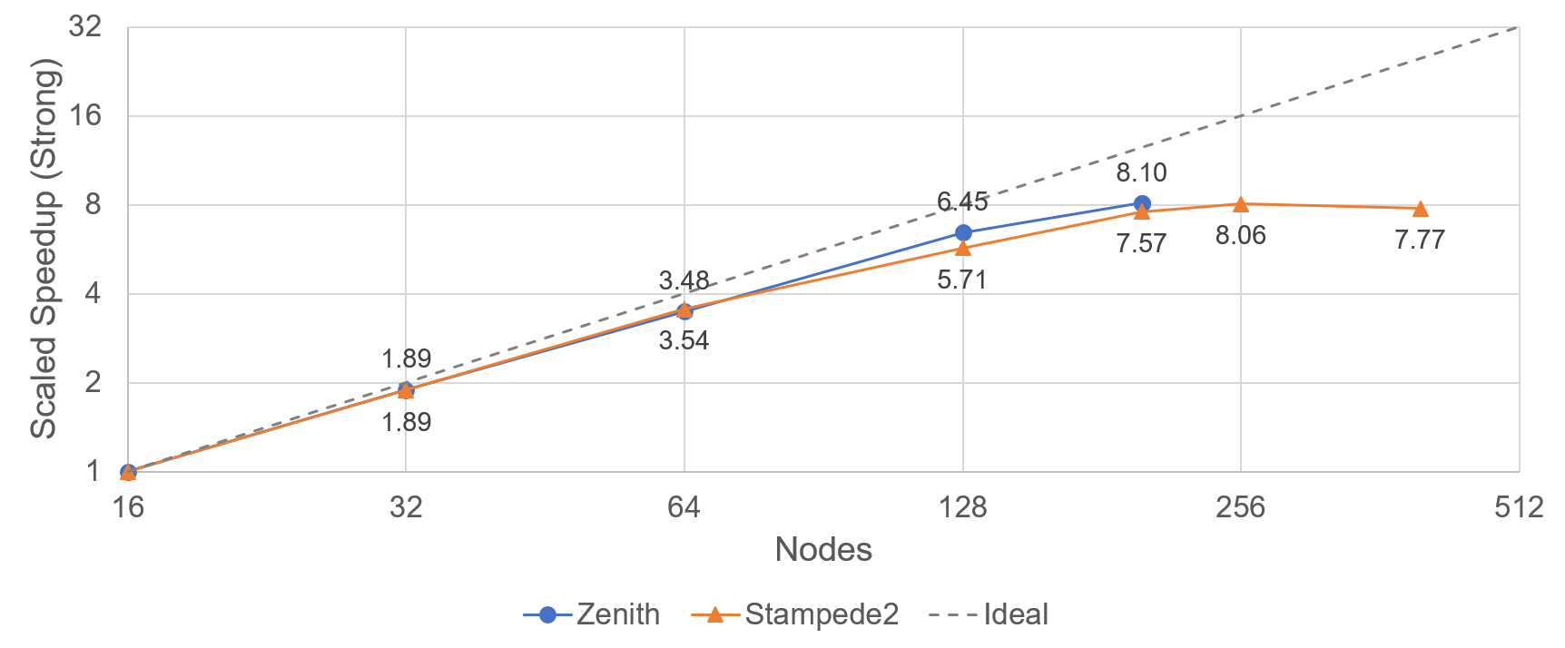
Figure 2: Scaled speedup (strong) performance.
Apart from the weak scaling performance benefit shown in our previous blog, the reduced gradient size also provides a way to perform efficient strong scaling. Figure 2 shows the strong scaling speedup performed on zenith and stampede2 supercomputers using up to 200 nodes on Zenith (Dell EMC) and 256 nodes on Stampede2 (TACC). Efficient strong scaling greatly helps to reduce the time to train the model
Diverged Training
While building a model quickly is important, it is critical the make sure that the resulting model is also accurate. Diverged training, where the produced model becomes less accurate (rather than more accurate) with continued training is a common problem not just for large batch training but in general for any NMT system. Monitoring the loss graph would help to understand the convergence of the deep learning model. Setting the learning rate to an optimal value is crucial for the model’s convergence.
Measures can be taken to prevent diverged training. Experiments suggest that having a very high learning rate at the beginning of the training would cause diverged training. But on the other hand, setting the learning rate too low also would make the model converge slowly. Finding the ideal learning rate for the model is therefore critical.
One solution is to reduce the learning rate (cool down or decay) or increase the learning rate (warm up), or more often a combination of both By allowing the learning rate to increase linearly to the set value for certain number of steps after which it decays based on a chosen function, the resulting model can be more accurate and produced faster. For transformer model, the decay is proportional to the inverse square root of the number of steps.

Figure 3: Learning rate decay used in Transformer model
Based on our experiments we found that for large batch sizes (130k, 402k, 630k, 1M tokens), setting the learning rate to 0.001 – 0.005 would prevent diverged training of the big model.
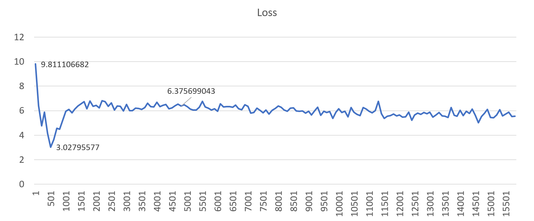
Figure 4: An example loss profile showing diverged training (gbz=130k, lr=0.01)
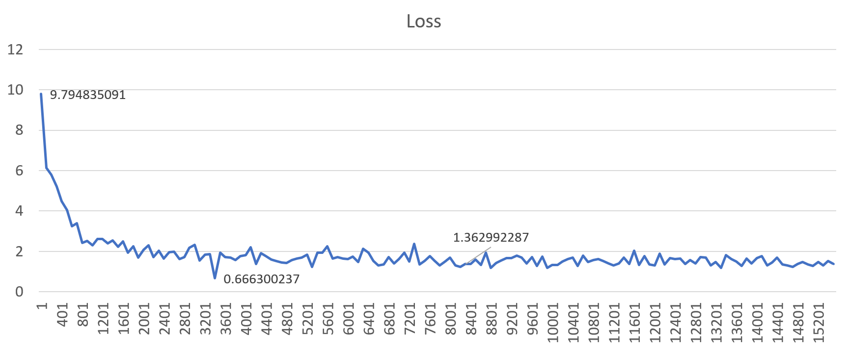
Figure 5: An example loss profile showing correct training behavior (gbz=130k, lr=0.001)
Figures 4 and 5 show the loss profiles when trained with a global batch size of 130k. Setting the learning rate to a “high” value (0.01) results in diverged training, but when set to 1e-3 (0.001), the model converges better. This results in good translation quality on the final model. Similar results were observed for all other large batch sizes.
Conclusion
In this blog, we highlighted a few common challenges when performing distributed training of the transformer model for neural machine translation (NMT). The solutions developed by Dell EMC in collaboration with Uber, Amazon, Intel, and SURFsara resulted in dramatically improved scaling capabilities and model accuracy. The results are now added part of our research paper accepted at the ISC High Performance 2019 conference. The paper has further details about the modifications to Horovod and improvements in terms of memory usage, scaling efficiency, reduced time to train and translation quality. The work has been incorporated into Horovod so that the research community can explore further scaling potential and produce more efficient NMT models.
Srinivas Varadharajan - Machine Learning/Deep Learning Developer
Twitter: @sedentary_yoda

Scaling Neural Machine Translation with Intel Xeon Scalable Processors
Mon, 12 Dec 2022 18:44:32 -0000
|Read Time: 0 minutes
The field of machine language translation is rapidly shifting from statistical machine learning models to efficient neural network architecture designs which can dramatically improve translation quality. However, training a better performing Neural Machine Translation (NMT) model still takes days to weeks depending on the hardware, size of the training corpus and the model architecture. Improving the time-to-solution for NMT training will be crucial if these approaches are to achieve mainstream adoption.
Intel® Xeon® Scalable processors are the workhorse of the modern datacenter, and over 90% of the Top500 super computers run on Intel. We can apply the supercomputing approach of scaling out to multiple servers to training NMT models in any datacenter. In this article we show some the effectiveness of and highlight important considerations when scaling a NMT model using Intel® Xeon® Scalable processors.
Encoder – decoder architecture
An NMT model reads a sentence in a source language and passes it to an encoder, which builds an intermediate representation. A decoder then processes the intermediate representation to produce a translated sentence in a target language.
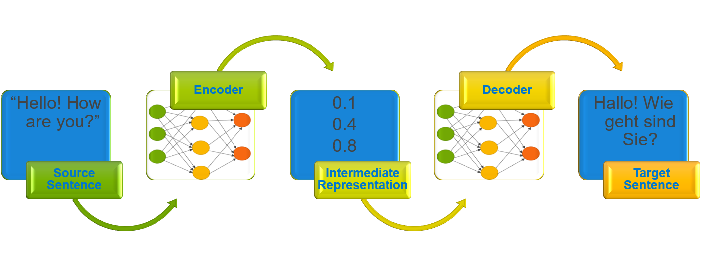
Figure 1: Encoder-decoder architecture
The figure above illustrates the encoder-decoder architecture. The English source sentence, “Hello! How are you?” is read and processed by the architecture to produce a translated German sentence “Hallo! Wie geht sind Sie?”. Traditionally, Recurrent Neural Network (RNN) was used in encoders and decoders, but other neural network architectures such as Convolutional Neural Network (CNN) and attention mechanism-based architectures are also used.
Architecture and environment
The Transformer model is one of the current architectures of interest in the field of NMT, and is built with variants of the attention mechanism which replace the traditional RNN components in the architecture. This architecture was able to produce a model that achieved state of the art results in English-German and English-French translation tasks.
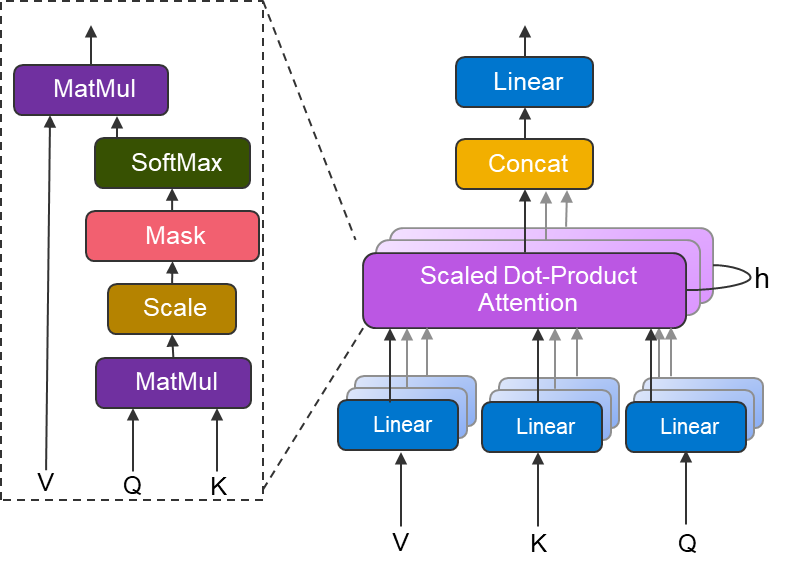
Figure 2: Multi-head attention block
The above figure shows the multi-head attention block used in the transformer architecture. At a high-level, the scaled dot-product attention can be thought as finding the relevant information, in the form of values (V) based on Query (Q) and Keys (K). Multi-head attention can be thought of as several attention layers in parallel, which together can identify distinct aspects of the input.
We use the Tensorflow official model implementation of the transformer architecture, which has been augmented with Uber’s Horovod distributed training framework. The training dataset used is the WMT English-German parallel corpus, which contains 4.5M English-German sentence pairs.
Our tests were performed in house on Zenith super computerin the Dell EMC HPC and AI Innovation lab. Zenith is a Dell EMC PowerEdge C6420-based cluster, consisting of 388 dual socket nodes powered by Intel® Xeon® Scalable Gold 6148 processors and interconnected with an Intel® Omni-path fabric.
System Information
CPU Model | Intel(R) Xeon(R) Gold 6148 CPU @ 2.40GHz |
Operating System | Red Hat Enterprise Linux Server release 7.4 (Maipo) |
Tensorflow Version | 1.10.1 with Intel® MKL |
Horovod Version | 0.15.0 |
MPI | Open MPI 3.1.2 |
Note: We used a specific Horovod branch to handle sparse gradients. Which is now part of the main branch in their GitHub repository.
Weak scaling, environment variables and TF configurations
When training using CPUs, environment variable settings and TensorFlow runtime configuration values play a vital role in improving the throughput and reducing the time to solution.
Below are the suggested settings based on our empirical tests when running 4 processes per node for the transformer (big) model on 50 zenith nodes.
Environment Variables
export OMP_NUM_THREADS=10 export KMP_BLOCKTIME=0 export KMP_AFFINITY=granularity=fine,verbose,compact,1,0 |
TF Configurations:
intra_op_parallelism_threads=$OMP_NUM_THREADS inter_op_parallelism_threads=1 |
Experimenting with weak scaling options allows finding the optimal number of processes run per node such that the model fits in the memory and performance doesn’t deteriorate. For some reason, TensorFlow creates an extra thread. Hence, to avoid oversubscription it’s better to set the OMP_NUM_THREADS to 9, 19 or 39 when training with 4,2,1 process per node respectively. Although we didn’t see it affecting the throughput performance in our experiments but may affect performance in a very large-scale setup.
Taking advantage of multi-threading can dramatically improve performance. This can be done by setting OMP_NUM_THREADS such that the product of its value and number of MPI ranks per node equals the number of available CPU cores per node. In the case of Zenith, this is 40 cores, as each PowerEdge C6420 node contains 2 20-core Intel® Xeon® Gold 6148 processors.
The KMP_AFFINITY environment variable provides a way to control the interface which binds OpenMP threads to physical processing units, while KMP_BLOCKTIME, sets the time in milliseconds that a thread should wait after completing a parallel execution before sleeping. TF configuration settings, intra_op_parallelism_threads, and inter_op_parallelism_threads are used to adjust the thread pools thereby optimizing the CPU performance.
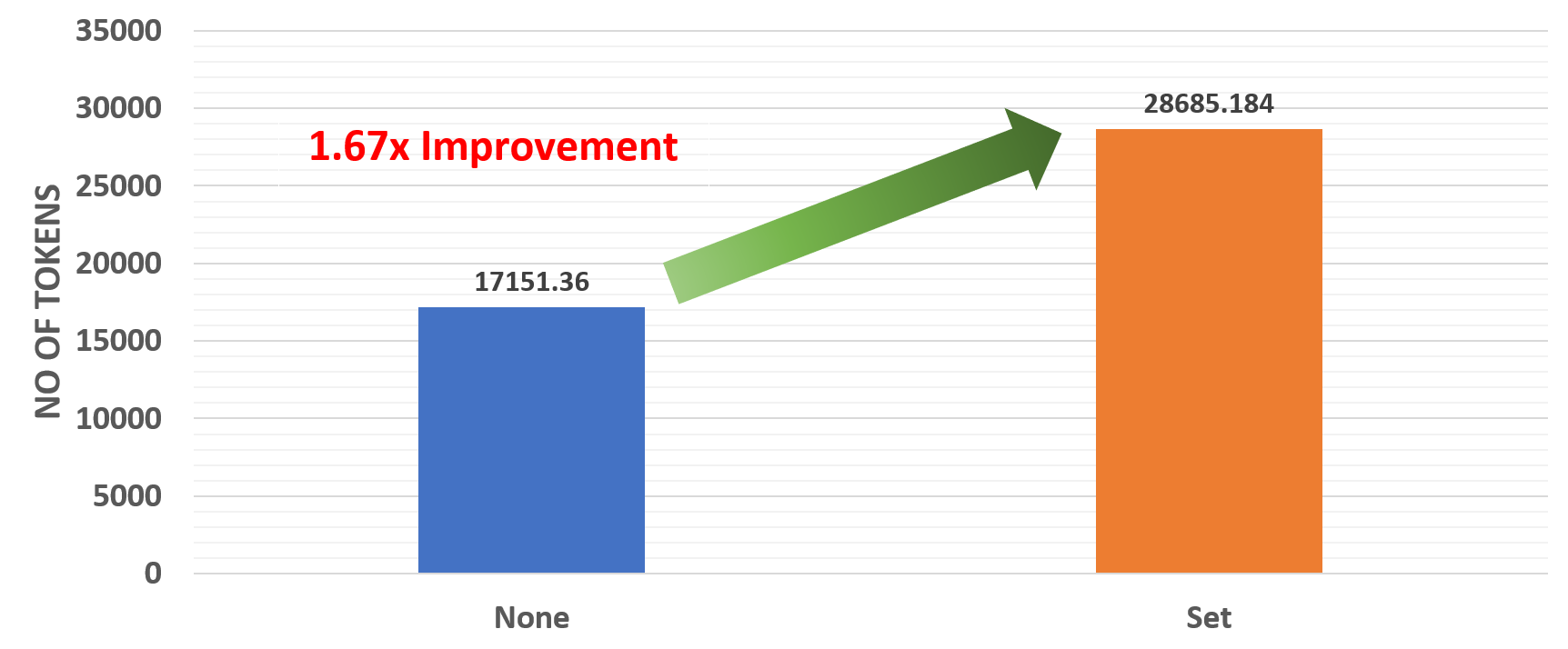
Figure 3: Effect of environment variables
The above results show that there’s a 1.67x improvement when environment variables are set correctly.
Faster distributed training
Training a large neural network architecture can be time-consuming, making it difficult to perform rapid prototyping or hyperparameter tuning. Thanks to distributed training and open source frameworks like Horovod, which allows training a model using multiple workers, the time to train can be substantially reduced. In our previous blog, we showed the effectiveness of training an AI radiologist with distributed deep learning and using Intel® Xeon® Scalable processors. Here, we show how distributed deep learning improves the time to train for machine translation models.
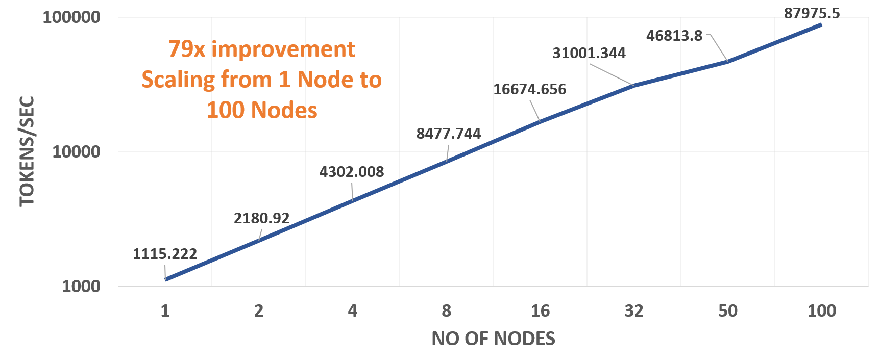
Figure 4: Scaling Performance
The above chart shows the throughput of the transformer (big) model when trained using up to 100 Zenith nodes. Our experiments show linear performance when scaling up the number of nodes. Based on our tests, which include setting the correct environment variables and the optimal number of MPI processes per node, we see a 79x improvement on 100 Zenith nodes with 2 processes per node compared to the throughput on a single node with 4 processes.
Translation Quality
NMT models’ translation quality is measured in terms of BLEU (Bi-Lingual Evaluation Understudy) score. It’s a measure to compute the difference between the human and machine-translated output.
In a previous blog post, we explained some of the challenges of large-batch training of deep learning models. Here, we experimented using a large global batch size of 402k tokens to determine the models’ accuracy on the English to German translation task. Hyperparameters were set to match those used for the transformer (big) model, and the model was trained using 50 Zenith nodes with 4 processes per node. The learning rate grows linearly for 4000 steps to 0.001 and then follows inverse square root decay.
Case-Insensitive BLEU | Case-Sensitive BLEU | |
TensorFlow Official Benchmark Results | 28.9 | - |
Our results | 29.15 | 28.56 |
Note: Case-Sensitive score not reported in the Tensorflow Official Benchmark.
The above table shows our results on the test set (newstest2014) after training the model for around 2.7 days (26000 steps). We can see a clear improvement in the translation quality compared to the results posted on the Tensorflow Official Benchmarks page. This shows that training with large batches does not adversely affect the quality of the resulting translation models, which is an encouraging result for future studies with even larger batch sizes.
Conclusion
In this post, we showed how to effectively train a Neural Machine Translation(NMT) system using Intel® Xeon® Scalable processors using distributed deep learning. We highlighted some of the best practices for setting environment variables and the corresponding scaling performance. Based on our experiments, and following other research work on NMT to understand some of the important aspects of scaling an NMT system, we were able to demonstrate better translation quality and accelerate the training process. With a research interest in the field of neural machine translation continuing to grow, we expect to see more interesting and innovative NMT architectures in the future.
Srinivas Varadharajan - Machine Learning/Deep Learning Developer
Twitter: @sedentary_yoda
LinkedIn: https://www.linkedin.com/in/srinivasvaradharajan

MLPerf™ v1.1 Inference on Virtualized and Multi-Instance GPUs

Mon, 16 May 2022 18:49:23 -0000
|Read Time: 0 minutes
Introduction
Graphics Processing Units (GPUs) provide exceptional acceleration to power modern Artificial Intelligence (AI) and Deep Learning (DL) workloads. GPU resource allocation and isolation are some of the key components that data scientists working in a shared environment use to run their DL experiments effectively. The need for this allocation and isolation becomes apparent when a single user uses only a small percentage of the GPU, resulting in underutilized resources. Due to the complexity of the design and architecture, maximizing the use of GPU resources in shared environments has been a challenge. The introduction of Multi-Instance GPU (MIG) capabilities in the NVIDIA Ampere GPU architecture provides a way to partition NVIDIA A100 GPUs and allow complete isolation between GPU instances. The Dell Validated Design showcases the benefits of virtualization for AI workloads and MIG performance analysis. This design uses the most recent version of VMware vSphere along with the NVIDIA AI Enterprise suite on Dell PowerEdge servers and VxRail Hyperconverged Infrastructure (HCI). Also, the architecture incorporates Dell PowerScale storage that supplies the required analytical performance and parallelism at scale to feed the most data-hungry AI algorithms reliably.
In this blog, we examine some key concepts, setup, and MLPerf Inference v1.1 performance characterization for VMs hosted on Dell PowerEdge R750xa servers configured with MIG profiles on NVIDIA A100 80 GB GPUs. We compare the inference results for the ResNet50 and Bidirectional Encoder Representations from Transformers (BERT) models.
Key Concepts
Key concepts include:
- Multi-Instance GPU (MIG)—MIG capability is an innovative technology released with the NVIDIA A100 GPU that enables partitioning of the A100 GPU up to seven instances or independent MIG devices. Each MIG device operates in parallel and is equipped with its own memory, cache, and streaming multiprocessors.
In the following figure, each block shows a possible MIG device configuration in a single A100 80 GB GPU:
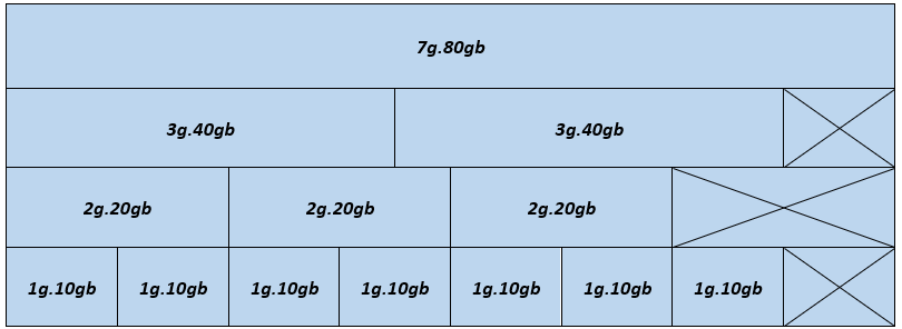
Figure 1- MIG device configuration - A100 80 GB GPU
The figure illustrates the physical location of GPU instances after they have been instantiated on the GPU. Because GPU instances are generated and destroyed at various locations, fragmentation might occur. The physical location of one GPU instance influences whether more GPU instances can be formed next to it.
Supported profiles for the A100 80GB GPU include:
- 1g.10gb
- 2g.20gb
- 3g.40gb
- 4g.40gb
- 7g.80gb
In Figure 1, a valid combination is constructed by beginning with an instance profile on the left and progressing to the right, ensuring that no two profiles overlap vertically. For detailed information about NVIDIA MIG profiles, see the NVIDIA Multi-Instance GPU User Guide.
- MLPERF—MLCommons™ is a consortium of leading researchers in AI from academia, research labs, and industry. Its mission is to "develop fair and useful benchmarks" that provide unbiased evaluations of training and inference performance for hardware, software, and services—all under controlled conditions. The foundation for MLCommons began with the MLPerf benchmark in 2018, which rapidly scaled as a set of industry metrics to measure machine learning performance and promote transparency of machine learning techniques. To stay current with industry trends, MLPerf is always evolving, conducting new tests, and adding new workloads that represent the state of the art in AI.
Setup for MLPerf Inference
A system under test consists of an ESXi host that can be operated from vSphere.
System details
The following table provides the system details.
Table 1: System details
Server | Dell PowerEdge R750xa (NVIDIA-Certified System) |
Processor | 2 x Intel Xeon Gold 6338 CPU @ 2.00 GHz |
GPU | 4 x NVIDIA A100 PCIe (PCI Express) 80 GB |
Network adapter | Mellanox ConnectX-6 Dual Port 100 GbE |
Storage | Dell PowerScale |
ESXi version | 7.0.3 |
BIOS version | 1.1.3 |
GPU driver version | 470.82.01 |
CUDA version | 11.4 |
System configuration for MLPerf Inference
The configuration for MLPerf Inference on a virtualized environment requires the following steps:
- Boot the host with ESXi (see Installing ESXi on the management hosts), install the NVIDIA bootbank driver, enable MIG, and restart the host.
- Create a virtual machine (VM) on the ESXi host with EFI boot mode (see Using GPUs with Virtual Machines on vSphere – Part 2: VMDirectPath I/O) and add the following advanced configuration settings:
pciPassthru.use64bitMMIO: TRUE
pciPassthru.allowP2P: TRUE
pciPassthru.64bitMMIOSizeGB: 64
- Change the VM settings and add a new PCIe device with a MIG profile (see Using GPUs with Virtual Machines on vSphere – Part 3: Installing the NVIDIA Virtual GPU Technology).
- Boot the Linux-based operating system and run the following steps in the VM.
- Install Docker, CMake (see Installing CMake), the build-essentials package, and CURL
- Download and install the NVIDIA MIG driver (grid driver).
- Install the nvidia-docker repository (see NVIDIA Container Toolkit Installation Guide) for running nvidia-containers.
- Configure the nvidia-grid service to use the vGPU setting on the VM (see Using GPUs with Virtual Machines on vSphere – Part 3: Installing the NVIDIA Virtual GPU Technology) and update the licenses.
- Run the following command to verify that the setup is successful:
nvidia-smi
Note: Each VM consists of 32 vCPUs and 64 GB memory.
MLPerf Inference configuration for MIG
When the system has been configured, configure MLPerf v1.1 on the MIG VMs. To run the MLPerf Inference benchmarks on a MIG-enabled system under test, do the following:
- Add MIG details in the inference configuration file:
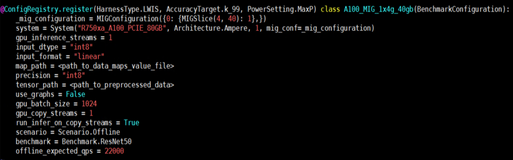 Figure 2- Example configuration for running inferences using MIG enabled VMs
 - Add valid MIG specifications to the system variable in the system_list.py file.
 Figure 3- Example system entry with MIG profiles
These steps complete the system setup, which is followed by building the image, generating engines, and running the benchmark. For detailed instructions, see our previous blog about running MLPerf v1.1 on bare metal systems.
MLPerf v1.1 Benchmarking
Benchmarking scenarios
We assessed inference latency and throughput for ResNet50 and BERT models using MLPerf Inference v1.1. The scenarios in the following table identify the number of VMs and corresponding MIG profiles used in performance tests. The total number of tests for each scenario is 57. The results are averaged based on three runs.
Note: We used MLPerf Inference v1.1 for benchmarking but the results shown in this blog are not part of the official MLPerf submissions.
Table 2: Scenarios configuration
Scenario | MIG profiles | Total VMs |
1 | MIG nvidia-7-80c | 1 |
2 | MIG nvidia-4-40c | 1 |
3 | MIG nvidia-3-40c | 1 |
4 | MIG nvidia-2-20c | 1 |
5 | MIG nvidia-1-10c | 1 |
6 | MIG nvidia-4-40c + nvidia-2-20c + nvidia-1-10c | 3 |
7 | MIG nvidia-2-20c + nvidia-2-20c + nvidia-2-20c + nvidia-1-10c | 4 |
8 | MIG nvidia-1-10c* 7 | 7 |
ResNet50
ResNet50 (see Deep Residual Learning for Image Recognition) is a widely used deep convolutional neural network for various computer vision applications. This neural network can address the disappearing gradients problem by allowing gradients to traverse the network's layers using the concept of skip connections. The following figure shows an example configuration for ResNet50 inference:
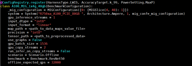
Figure 4- Configuration for running inference using Resnet50 model
The following figure shows ResNet50 inference performance based on the scenarios in Table 2: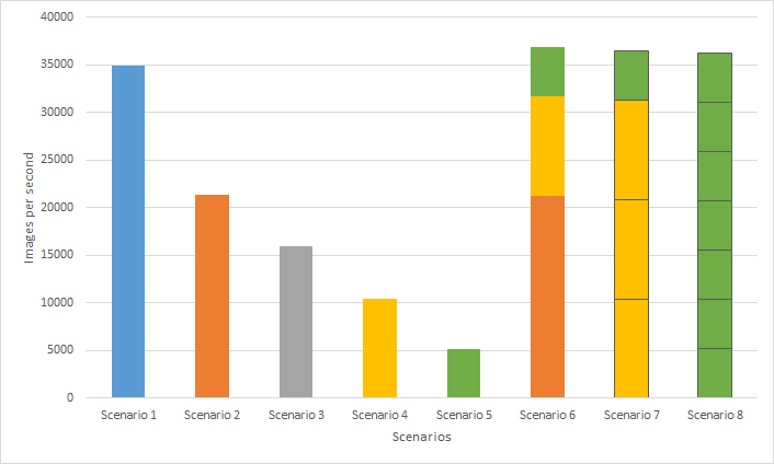
Figure 5- ResNet50 Performance throughput of MLPerf Inference v1.1 across various VMs with MIG profiles
Multiple data scientists can use all the available GPU resources while running their individual workloads on separate instances, improving overall system throughput. This result is clearly seen on Scenarios 6 through 8, which contain multiple instances, compared to Scenario 1 which consists of a single instance with the largest MIG profile for A100 80 GB. Scenario 6 achieves the highest overall system throughput (5.77 percent improvement) compared to Scenario 1. Also, Scenario 8 shows seven VMs equipped with individual GPU instances that can be built for up to seven data scientists who can fine-tune their ResNet50 base models.
BERT
BERT (see BERT: Pre-training of Deep Bidirectional Transformers for Language Understanding) is a state-of-the-art language representational model. BERT is essentially a stack of Transformer encoders. It is suitable for neural machine translation, question answering, sentiment analysis, and text summarization, all of which require a working knowledge of the target language.
BERT is trained in two stages:
- Pretrain—During which the model acquires language and context understanding
- Fine-tuning—During which the model acquires task-specific knowledge such as querying and response.
The following figure shows an example configuration for BERT inference:
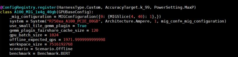
Figure 6- Configuration for running inference using BERT model
The following figure shows BERT inference performance based on scenarios in Table 2:
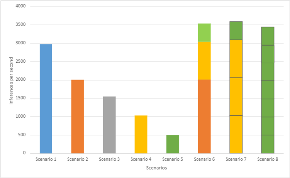 Figure 7- BERT Performance throughput of MLPerf Inference v1.1 across various VMs with MIG profiles
Like Resnet50 Inference performance, we clearly see that Scenarios 6 through 8, which contain multiple instances, perform better compared to Scenario 1. Particularly, Scenario 7 achieves the highest overall system throughput (21 percent improvement) compared to Scenario 1 while achieving 99.9 percent accuracy target. Also, Scenario 8 shows seven VMs equipped with individual GPU instances that can be built for up to seven data scientists who want to fine-tune their BERT base models.
Conclusion
In this blog, we describe how to install and configure MLPerf Inference v1.1 on Dell PowerEdge 750xa servers using a VMware-virtualized infrastructure and NVIDIA A100 GPUs. Furthermore, we examine the performance of single- and multi-MIG profiles running on the A100 GPU. If your ML workload is primarily inferencing-focused and response time is not an issue, enabling MIG on the A100 GPU can ensure complete GPU use with maximum throughput. Developers can use VMs with an independent GPU compute allocated to them. Also, in cases where the largest MIG profiles are used, performance is comparable to bare metal systems. Inference results from ResNet50 and BERT models demonstrate that overall system performance using either the whole GPU or multiple VMs with MIG instances hosted on an R750xa system with VMware ESXi and NVIDIA A100 GPUs performed well and produced valid results for MLPerf Inference v1.1. In both the cases, the average throughput and latency are equal. This result confirms that MIG provides predictable latency and throughput independent of other processes operating on the MIG instances on the GPU.
There is a MIG limitation for GPU profiling on the VMs. Due to the shared nature of the hardware performance across all MIG devices, only one GPU profiling session can run on a VM; parallel GPU profiling sessions on a single VM are not possible.

Accelerating Distributed Training in a Multinode Virtualized Environment
Fri, 13 May 2022 13:57:13 -0000
|Read Time: 0 minutes
Introduction
In the age of deep learning (DL), with complex models, it is vital to have a system that allows faster distributed training. Depending on the application, some DL models require more frequent retraining and fine-tuning of the hyperparameters to be deployed in the production environment. It is important to understand the best practices to improve multinode distributed training performance.
Networking is critical in a distributed training setup as there are numerous gradients exchanged between the nodes. The complexity increases as we increase the number of nodes. In the past, we have seen the benefits of using:
- Direct Memory Access (DMA), which enables a device to access host memory without the intervention of CPUs
- Remote Direct Memory Access (RDMA), which enables access to memory on a remote machine without interrupting the CPU processes on that system
This blog examines performance when direct communication is established between the GPUs in multinode training experiments run on Dell PowerEdge servers with NVIDIA GPUs and VMware vSphere.
GPUDirect RDMA
Introduced as part of Kepler class GPUs and CUDA 5.0, GPUDirect RDMA enables a direct communication path between NVIDIA GPUs and third-party devices such as network interfaces. By establishing direct communication between the GPUs, we can eliminate the critical bottleneck where data needs to be moved into the host system memory before it can be sent over the network, as shown in the following figure:
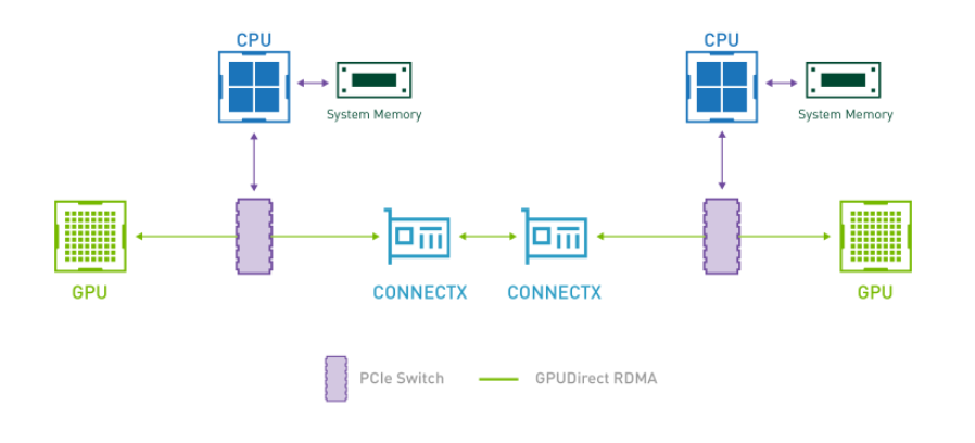
Figure 1: Direct Communication – GPUDirect RDMA
For more information, see:
System details
The following table provides the system details:
Table 1: System details
Component | Details |
Server | Dell PowerEdge R750xa (NVIDIA-Certified System) |
Processor | 2 x Intel Xeon Gold 6338 CPU @ 2.00 GHz |
GPU | 4 x NVIDIA A100 PCIe |
Network adapters | Mellanox ConnectX-6 Dual port 100 GbE and 25 GbE |
Storage | Dell PowerScale |
ESXi version | 7.0.3 |
BIOS version | 1.1.3 |
GPU driver version | 470.82.01 |
CUDA Version | 11.4 |
Setup
The setup for multinode training in a virtualized environment is outlined in our previous blog.
At a high level, after Address Translation Services (ATS) is enabled on VMware ESXi, the VMs, and ConnectX-6 NIC:
- Enable mapping between logical and physical ports.
- Create a Docker container with Mellanox OFED drivers, Open MPI Library, and NVIDIA-optimized TensorFlow.
- Set up a keyless SSH login between VMs
Performance evaluation
For evaluation, we use tf_cnn_benchmarks using the ResNet50 model and synthetic data with a local batch size of 1024. Each VM is configured with 32 vCPUs, 64 GB of memory, and one NVIDIA A100 PCIE 80 GB GPU. The experiments are performed by using a data parallelism approach in a distributed training setup, scaling up to four nodes. The results are based on averaging three experiment runs. Single-node experiments are only for comparison as there is no internode communication.
Note: Use the ibdev2netdev utility to display the installed Mellanox ConnectX-6 card along with the mapping of ports. In the following figures, ON and OFF indicate if the mapping is enabled between logical and physical ports.
The following figure shows performance when scaling up to four nodes using Mellanox ConnectX-6 Dual Port 100 GbE. It is clear that the throughput increases significantly when the mapping is enabled (ON), providing direct communication between NVIDIA GPUs. The two-node experiments show an improvement in throughput of 18.7 percent while the four node experiments improve throughput by 26.7 percent.
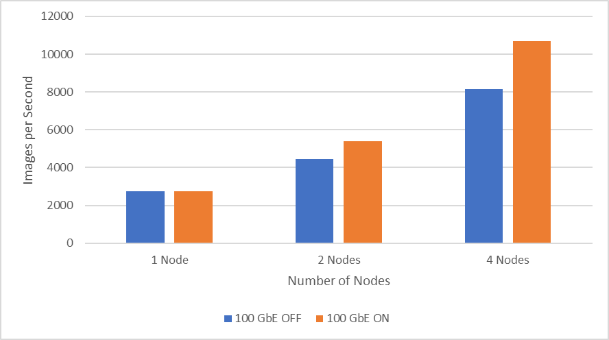
Figure 2: 100 GbE network performance
The following figure shows the scaling performance comparison between Mellanox ConnectX-6 Dual Port 100 GbE and Mellanox ConnectX-6 Dual Port 25 GbE while performing distributed training of the ResNet50 model. Using 100 GbE, two-node experiment results show an improved throughput of six percent while four-node experiments show an improved performance of 11.6 percent compared to 25 GbE.
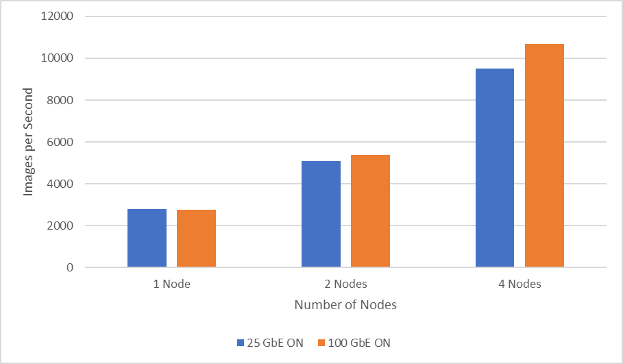
Figure 3: 25 GbE compared to 100 GbE network performance
Conclusion
In this blog, we considered GPUDirect RDMA and a few required steps to setup multinode experiments in the virtualized environment. The results showed that scaling to a larger number of nodes boosts throughput significantly when establishing direct communication between GPUs in a distributed training setup. The blog also showcased the performance comparison between Mellanox ConnectX-6 Dual Port 100 GbE and 25 GbE network adapters used for distributed training of a ResNet50 model.