


Running the MLPerf™ Inference v1.1 Benchmark on Dell EMC Systems
Fri, 24 Sep 2021 16:51:50 -0000
|Read Time: 0 minutes
Related Blog Posts

MLPerf™ Inference v4.0 Performance on Dell PowerEdge R760xa and R7615 Servers with NVIDIA L40S GPUs
Fri, 05 Apr 2024 17:41:56 -0000
|Read Time: 0 minutes
Abstract
Dell Technologies recently submitted results to the MLPerf™ Inference v4.0 benchmark suite. This blog highlights Dell Technologies’ closed division submission made for the Dell PowerEdge R760xa, Dell PowerEdge R7615, and Dell PowerEdge R750xa servers with NVIDIA L40S and NVIDIA A100 GPUs.
Introduction
This blog provides relevant conclusions about the performance improvements that are achieved on the PowerEdge R760xa and R7615 servers with the NVIDIA L40S GPU compared to the PowerEdge R750xa server with the NVIDIA A100 GPU. In the following comparisons, we held the GPU constant across the PowerEdge R760xa and PowerEdge R7615 servers to show the excellent performance of the NVIDIA L40S GPU. Additionally, we also compared the PowerEdge R750xa server with the NVIDIA A100 GPU to its successor the PowerEdge R760xa server with the NVIDIA L40S GPU.
System Under Test configuration
The following table shows the System Under Test (SUT) configuration for the PowerEdge servers.
Table 1: SUT configuration of the Dell PowerEdge R750xa, R760xa, and R7615 servers for MLPerf Inference v4.0
Server | PowerEdge R750xa | PowerEdge R760xa | PowerEdge R7615 |
MLPerf Version | V4.0
| ||
GPU | NVIDIA A100 PCIe 80 GB | NVIDIA L40S
| |
Number of GPUs | 4 | 2 | |
MLPerf System ID | R750xa_A100_PCIe_80GBx4_TRT | R760xa_L40Sx4_TRT | R7615_L40Sx2_TRT
|
CPU | 2 x Intel Xeon Gold 6338 CPU @ 2.00GHz | 2 x Intel Xeon Platinum 8470Q | 1 x AMD EPYC 9354 32-Core Processor |
Memory | 512 GB | ||
Software Stack | TensorRT 9.3.0 CUDA 12.2 cuDNN 8.9.2 Driver 535.54.03 / 535.104.12 DALI 1.28.0 | ||
The following table lists the technical specifications of the NVIDIA L40S and NVIDIA A100 GPUs.
Table 2: Technical specifications of the NVIDIA A100 and NVIDIA L40S GPUs
Model | NVIDIA A100 | NVIDIA L40S | ||
Form factor | SXM4 | PCIe Gen4 | PCIe Gen4 | |
GPU architecture | Ampere | Ada Lovelace | ||
CUDA cores | 6912 | 18176 | ||
Memory size | 80 GB | 48 GB | ||
Memory type | HBM2e | HBM2e | ||
Base clock | 1275 MHz | 1065 MHz | 1110 MHz | |
Boost clock | 1410 MHz | 2520 MHz | ||
Memory clock | 1593 MHz | 1512 MHz | 2250 MHz | |
MIG support | Yes | No | ||
Peak memory bandwidth | 2039 GB/s | 1935 GB/s | 864 GB/s | |
Total board power | 500 W | 300 W | 350 W | |
Dell PowerEdge R760xa server
The PowerEdge R760xa server shines as an Artificial Intelligence (AI) workload server with its cutting-edge inferencing capabilities. This server represents the pinnacle of performance in the AI inferencing space with its processing prowess enabled by Intel Xeon Platinum processors and NVIDIA L40S GPUs. Coupled with NVIDIA TensorRT and CUDA 12.2, the PowerEdge R760xa server is positioned perfectly for any AI workload including, but not limited to, Large Language Models, computer vision, Natural Language Processing, robotics, and edge computing. Whether you are processing image recognition tasks, natural language understanding, or deep learning models, the PowerEdge R760xa server provides the computational muscle for reliable, precise, and fast results.
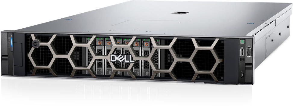
Figure 1: Front view of the Dell PowerEdge R760xa server

Figure 2: Top view of the Dell PowerEdge R760xa server
Dell PowerEdge R7615 server
The PowerEdge R7615 server stands out as an excellent choice for AI, machine learning (ML), and deep learning (DL) workloads due to its robust performance capabilities and optimized architecture. With its powerful processing capabilities including up to three NVIDIA L40S GPUs supported by TensorRT, this server can handle complex neural network inference and training tasks with ease. Powered by a single AMD EPYC processor, this server performs well for any demanding AI workloads.
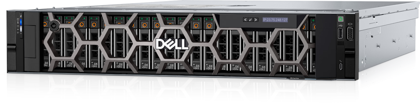
Figure 3: Front view of the Dell PowerEdge R7615 server
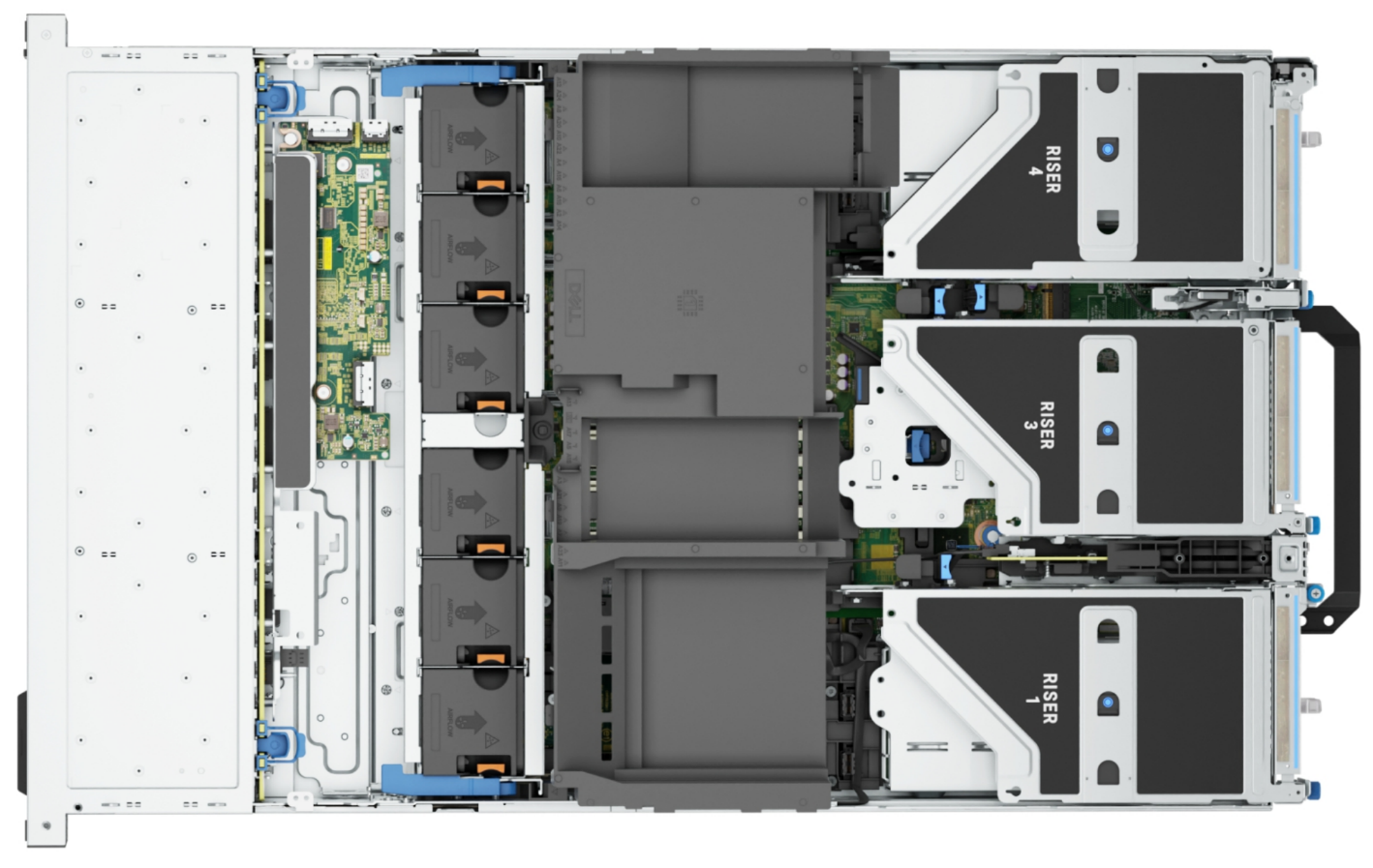
Figure 4: Top view of the Dell PowerEdge R7615 server
Dell PowerEdge R750xa server
The PowerEdge R750xa server is a perfect blend of technological prowess and innovation. This server is equipped with Intel Xeon Gold processors and the latest NVIDIA GPUs. The PowerEdge R760xa server is designed for the most demanding AI, ML, and DL workloads as it is compatible with the latest NVIDIA TensorRT engine and CUDA version. With up to nine PCIe Gen4 slots and availability in a 1U or 2U configuration, the PowerEdge R750xa server is an excellent option for any demanding workload.
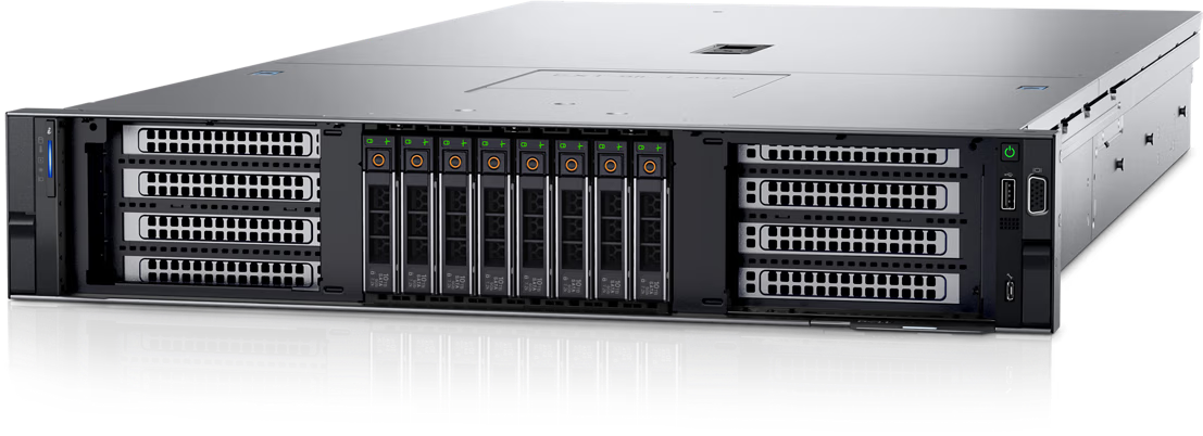
Figure 5: Front view of the Dell PowerEdge R750xa server
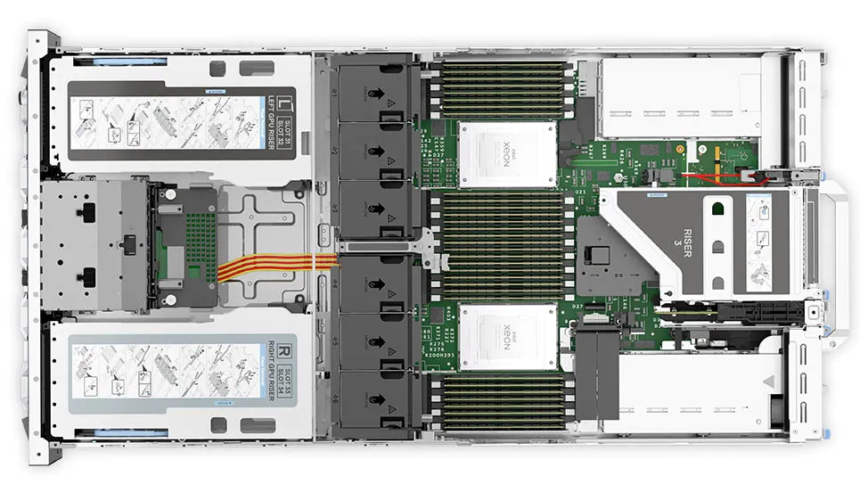
Figure 6: Top view of the Dell PowerEdge R750xa server
Performance results
Classical Deep Learning models performance
The following figure presents the results as a ratio of normalized numbers over the Dell PowerEdge R750xa server with four NVIDIA A100 GPUs. This result provides an easy-to-read comparison of three systems and several benchmarks.
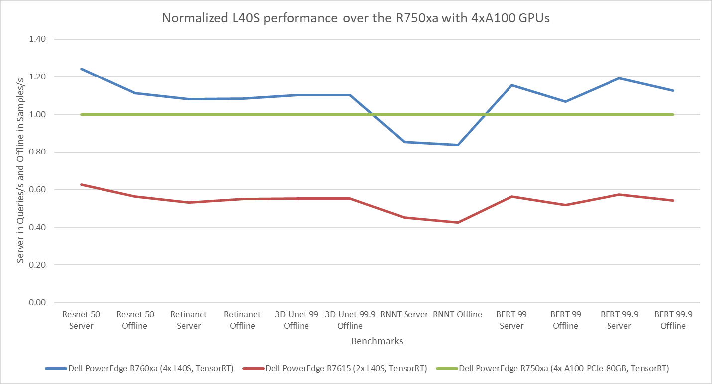
Figure 7: Normalized NVIDIA L40S GPU performance over the PowerEdge R750xa server with four A100 GPUs
The green trendline represents the performance of the Dell PowerEdge R750xa server with four NVIDIA A100 GPUs. With a score of 1.00 for each benchmark value, the results have been divided by themselves to serve as the baseline in green for this comparison. The blue trendline represents the performance of the PowerEdge R760xa server with four NVIDIA L40S GPUs that has been normalized by dividing each benchmark result by the corresponding score achieved by the PowerEdge R750xa server. In most cases, the performance achieved on the PowerEdge R760xa server outshines the results of the PowerEdge R750xa server with NVIDIA A100 GPUs, proving the expected improvements from the NVIDIA L40S GPU. The red trendline has also been normalized over the PowerEdge R750xa server and represents the performance of the PowerEdge R7615 server with two NVIDIA L40S GPUs. It is interesting that the red line almost mimics the blue line. This result suggests that the PowerEdge R7615 server, despite having half the compute resources, still performs comparably well in most cases, showing its efficiency.
Generative AI performance
The latest submission saw the introduction of the new Stable Diffusion XL benchmark. In the context of generative AI, stable diffusion is a text to image model that generates coherent image samples. This result is achieved gradually by refining and spreading out information throughout the generation process. Consider the example of dropping food coloring into a large bucket of water. Initially, only a small, concentrated portion of the water turns color, but gradually the coloring is evenly distributed in the bucket.
The following table shows the excellent performance of the PowerEdge R760xa server with the powerful NVIDIA L40S GPU for the GPT-J and Stable Diffusion XL benchmarks. The PowerEdge R760xa takes the top spot in GPT-J and Stable Diffusion XL when compared to other NVIDIA L40S results.
Table 3: Benchmark results for the PowerEdge R760xa server with the NVIDIA L40S GPU
Benchmark | Dell PowerEdge R760xa L40S result (Server in Queries/s and Offline in Samples/s) | Dell’s % gain to the next best non-Dell results (%) |
Stable Diffusion XL Server | 0.65 | 5.24 |
Stable Diffusion XL Offline | 0.67 | 2.28 |
GPT-J 99 Server | 12.75 | 4.33 |
GPT-J 99 Offline | 12.61 | 1.88 |
GPT-J 99.9 Server | 12.75 | 4.33 |
GPT-J 99.9 Offline | 12.61 | 1.88 |
Conclusion
The MLPerf Inference submissions elicit insightful like-to-like comparisons. This blog highlights the impressive performance of the NVIDIA L40S GPU in the Dell PowerEdge R760xa and PowerEdge R7615 servers. Both servers performed well when compared to the performance of the Dell PowerEdge R750xa server with the NVIDIA A100 GPU. The outstanding performance improvements in the NVIDIA L40S GPU coupled with the Dell PowerEdge server position Dell customers to succeed in AI workloads. With the advent of the GPT-J and Stable diffusion XL Models, the Dell PowerEdge server is well positioned to handle Generative AI workloads.

Dell PowerEdge Servers Unleash Another Round of Excellent Results with MLPerf™ v4.0 Inference
Wed, 27 Mar 2024 15:12:53 -0000
|Read Time: 0 minutes
Today marks the unveiling of MLPerf v4.0 Inference results, which have emerged as an industry benchmark for AI systems. These benchmarks are responsible for assessing the system-level performance consisting of state-of-the-art hardware and software stacks. The benchmarking suite contains image classification, object detection, natural language processing, speech recognition, recommenders, medical image segmentation, LLM 6B and LLM 70B question answering, and text to image benchmarks that aim to replicate different deployment scenarios such as the data center and edge.
Dell Technologies is a founding member of MLCommons™ and has been actively making submissions since the inception of the Inference and Training benchmarks. See our MLPerf™ Inference v2.1 with NVIDIA GPU-Based Benchmarks on Dell PowerEdge Servers white paper that introduces the MLCommons Inference benchmark.
Our performance results are outstanding, serving as a clear indicator of our resolve to deliver outstanding system performance. These improvements enable higher system performance when it is most needed, for example, for demanding generative AI (GenAI) workloads.
What is new with Inference 4.0?
Inference 4.0 and Dell’s submission include the following:
- Newly introduced Llama 2 question answering and text to image stable diffusion benchmarks, and submission across different Dell PowerEdge XE platforms.
- Improved GPT-J (225 percent improvement) and DLRM-DCNv2 (100 percent improvement) performance. Improved throughput performance of the GPTJ and DLRM-DCNv2 workload means faster natural language processing tasks like summarization and faster relevant recommendations that allow a boost to revenue respectively.
- First-time submission of server results with the recently released PowerEdge R7615 and PowerEdge XR8620t servers with NVIDIA accelerators.
- Besides accelerator-based results, Intel-based CPU-only results.
- Results for PowerEdge servers with Qualcomm accelerators.
- Power results showing high performance/watt scores for the submissions.
- Virtualized results on Dell servers with Broadcom.
Overview of results
Dell Technologies delivered 187 data center, 28 data center power, 42 edge, and 24 edge power results. Some of the more impressive results were generated by our:
- Dell PowerEdge XE9680, XE9640, XE8640, and servers with NVIDIA H100 Tensor Core GPUs
- Dell PowerEdge R7515, R750xa, and R760xa servers with NVIDIA L40S and A100 Tensor Core GPUs
- Dell PowerEdge XR7620 and XR8620t servers with NVIDIA L4 Tensor Core GPUs
- Dell PowerEdge R760 server with Intel Emerald Rapids CPUs
- Dell PowerEdge R760 with Qualcomm QAIC100 Ultra accelerators
NVIDIA-based results include the following GPUs:
- Eight-way NVIDIA H100 GPU (SXM)
- Four-way NVIDIA H100 GPU (SXM)
- Four-way NVIDIA A100 GPU (PCIe)
- Four-way NVIDIA L40S GPU (PCIe)
- NVIDIA L4 GPU
These accelerators were benchmarked on different servers such as PowerEdge XE9680, XE8640, XE9640, R760xa, XR7620, and XR8620t servers across data center and edge suites.
Dell contributed to about 1/4th of the closed data center and edge submissions. The large number of result choices offers end users an opportunity to make data-driven purchase decisions and set performance and data center design expectations.
Interesting Dell data points
The most interesting data points include:
- Performance results across different benchmarks are excellent and show that Dell servers meet the increasing need to serve different workload types.
- Among 20 submitters, Dell Technologies was one of the few companies that covered all benchmarks in the closed division for data center suites.
- The PowerEdge XE8640 and PowerEdge XE9640 servers compared to other four-way systems procured winning titles across all the benchmarks including the newly launched stable diffusion and Llama 2 benchmark.
- The PowerEdge XE9680 server compared to other eight-way systems procured several winning titles for benchmarks such as ResNet Server, 3D-Unet, BERT-99, and BERT-99.9 Server.
- The PowerEdge XE9680 server delivers the highest performance/watt compared to other submitters with 8-way NVIDIA H100 GPUs for ResNet Server, GPTJ Server, and Llama 2 Offline
- The Dell XR8620t server for edge benchmarks with NVIDIA L4 GPUs outperformed other submissions.
- The PowerEdge R750xa server with NVIDIA A100 PCIe GPUs outperformed other submissions on the ResNet, RetinaNet, 3D-Unet, RNN-T, BERT 99.9, and BERT 99 benchmarks.
- The PowerEdge R760xa server with NVIDIA L40S GPUs outperformed other submissions on the ResNet Server, RetinaNet Server, RetinaNet Offline, 3D-UNet 99, RNN-T, BERT-99, BERT-99.9, DLRM-v2-99, DLRM-v2-99.9, GPTJ-99, GPTJ-99.9, Stable Diffusion XL Server, and Stable Diffusion XL Offline benchmarks.
Highlights
The following figure shows the different Offline and Server performance scenarios in the data center suite. These results provide an overview; follow-up blogs will provide more details about the results.
The following figure shows that these servers delivered excellent performance for all models in the benchmark such as ResNet, RetinaNet, 3D-UNet, RNN-T, BERT, DLRM-v2, GPT-J, Stable Diffusion XL, and Llama 2. Note that different benchmarks operate on varied scales. They have all been showcased in an exponentially scaled y-axis in the following figure:
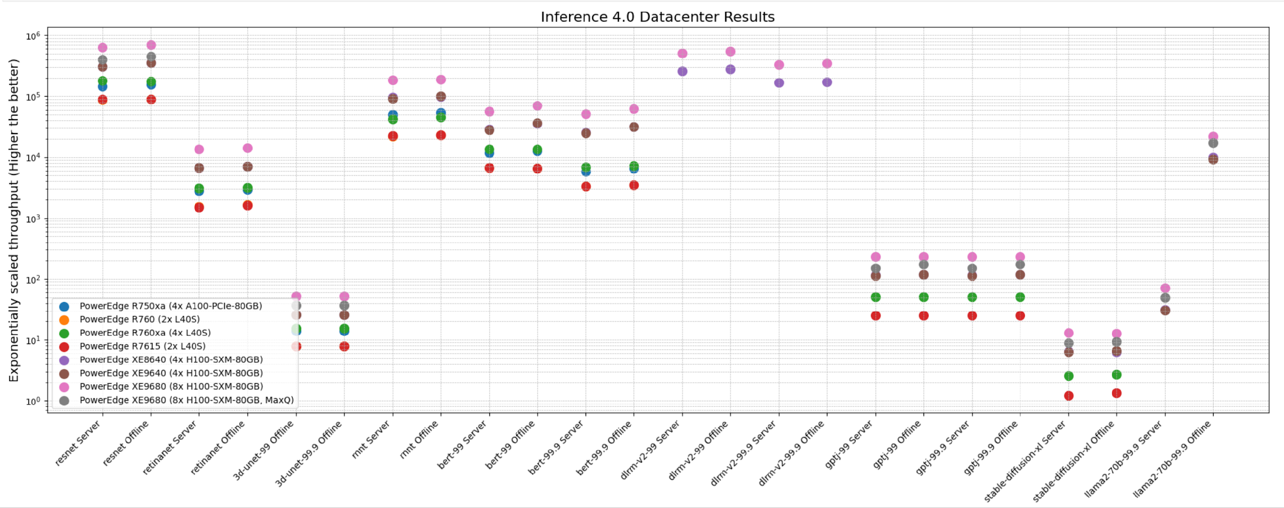
Figure 1: System throughput for submitted systems for the data center suite.
The following figure shows single-stream and multistream scenario results for the edge for ResNet, RetinaNet, 3D-Unet, RNN-T, BERT 99, GPTJ, and Stable Diffusion XL benchmarks. The lower the latency, the better the results and for Offline scenario, higher the better.
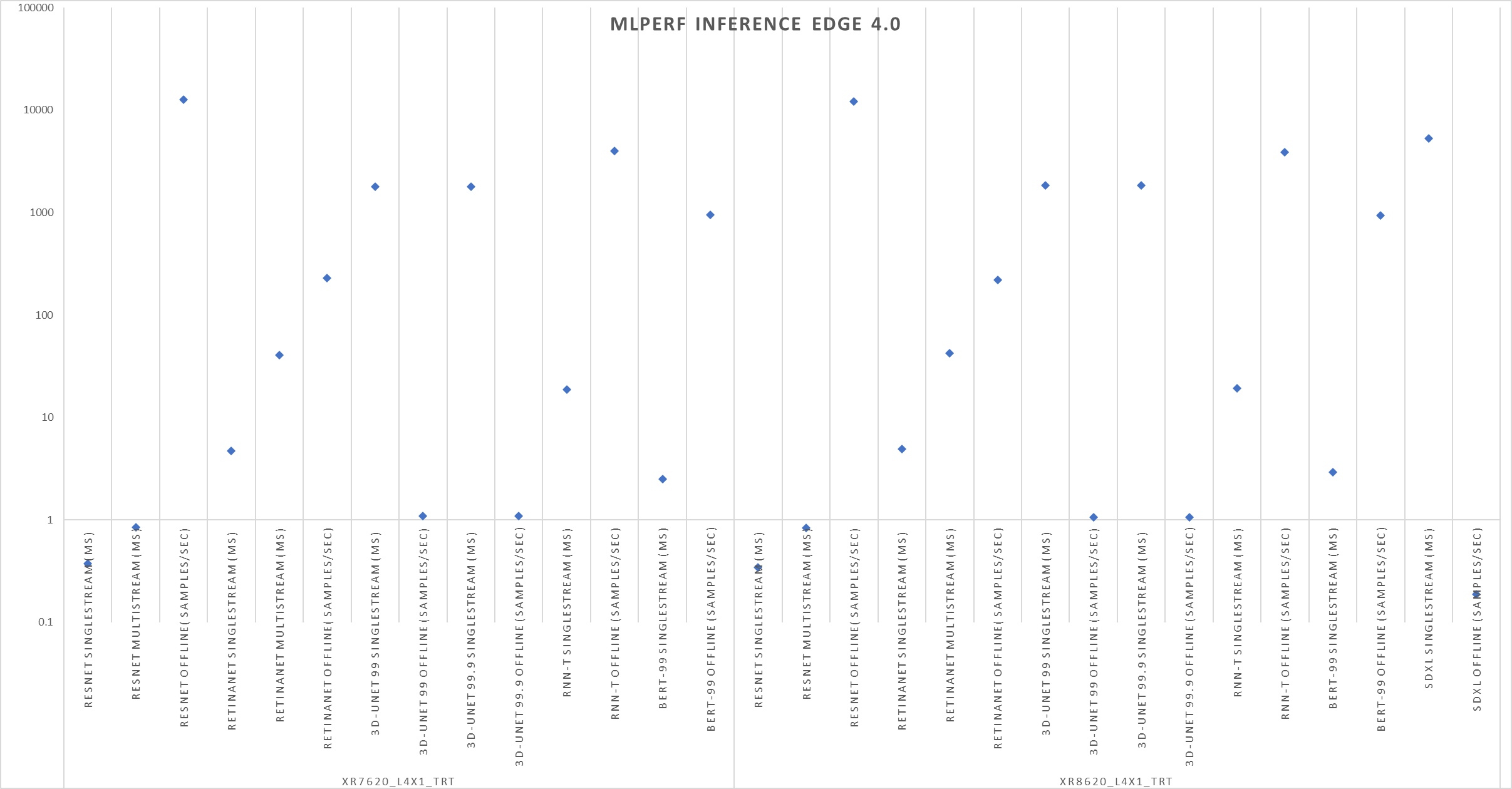
Figure 2: Edge results with PowerEdge XR7620 and XR8620t servers overview
Conclusion
The preceding results were officially submitted to MLCommons. They are MLPerf-compliant results for the Inference v4.0 benchmark across various benchmarks and suites for all the tasks in the benchmark such as image classification, object detection, natural language processing, speech recognition, recommenders, medical image segmentation, LLM 6B and LLM 70B question answering, and text to image. These results prove that Dell PowerEdge XE9680, XE8640, XE9640, and R760xa servers are capable of delivering high performance for inference workloads. Dell Technologies secured several #1 titles that make Dell PowerEdge servers an excellent choice for data center and edge inference deployments. End users can benefit from the plethora of submissions that help make server performance and sizing decisions, which ultimately deliver enterprises’ AI transformation and shows Dell’s commitment to deliver higher performance.
MLCommons Results
https://mlcommons.org/en/inference-datacenter-40/
https://mlcommons.org/en/inference-edge-40/
The preceding graphs are MLCommons results for MLPerf IDs from 4.0-0025 to 4.0-0035 on the closed datacenter, 4.0-0036 to 4.0-0038 on the closed edge, 4.0-0033 in the closed datacenter power, and 4.0-0037 in closed edge power.