


LAMMPS — with Ice Lake on Dell EMC PowerEdge Servers
3rd Generation Intel Xeon® Scalable processors (architecture code named Ice Lake) is Intel’s successor to Cascade Lake. New features include up to 40 cores per processor, eight memory channels with support for 3200 MT/s memory speed and PCIe Gen4. The HPC and AI Innovation Lab at Dell EMC had access to a few systems and this blog presents the results of our initial benchmarking study.
LAMMPS Overview
Large-scale Atomic/Molecular Massively Parallel Simulator (LAMMPS) is an open source, well parallelized collection of packages for molecular dynamics (MD) research. LAMMPS has a nice collection of “atom styles”, force fields, and many contributed packages. LAMMPS can run on a single processor or on the largest parallel super-computers. It also has packages that provide force calculations accelerated on GPU’s. It can do simulations with billions of atoms!
LAMMPS can be run on a single processor or in parallel using some form of message passing, such as Message Passing Interface (MPI). The most current source code for LAMMPS is written in C++. For more information about LAMMPS, see the following link: https://www.lammps.org/.
Objective
In this study we measure the performance of LAMMPS on different Ice Lake processor models as listed in Table 1 with a comparison to the previous generation Cascade Lake systems. Single node as well as the multi-node scalability tests were conducted.
Compilation Details
The LAMMPS version used for testing release was lammps-2July-2021, using the Intel 2020 update 5 compiler to take advantage of AVX2 and AVX512 optimizations, and the Intel MKL FFT library. We used the default INTEL package, which comes along the LAMMPS package providing some well optimized atom pair styles in LAMMPS for the vector instructions on Intel processors. The datasets used for our study are described in Table 2, along with detailed configuration of atom sizes and run steps. The unit of performance is timesteps per second, and higher is better.
Hardware and software configurations
Table 1: Hardware and Software test bed details
Component | Dell EMC PowerEdge R750 server | Dell EMC PowerEdge R750 server | Dell EMC PowerEdge C6520 server | Dell EMC PowerEdge C6520 server | Dell EMC PowerEdge C6420 server | Dell EMC PowerEdge C6420 server |
CPU model | Xeon 8380 | Xeon 8358 | Xeon 8352Y | Xeon 6330 | Xeon 8280 | Xeon 6248R |
Cores/Socket | 40 | 32 | 32 | 28 | 28 | 24 |
Base Frequency | 2.30 GHz | 2.60 GHz | 2.20 GHz | 2.00 GHz | 2.70 GHz | 3.00 GHz |
TDP | 270 W | 250 W | 205 W | 205 W | 205 W | 205 W |
Operating System | Red Hat Enterprise Linux 8.3 4.18.0-240.22.1.el8_3.x86_64 | |||||
Memory |
16 GB x 16 (2Rx8) 3200 MT/s
| 16 GB x 12 (2Rx8) 2933 MT/s | ||||
BIOS/CPLD | 1.1.2/1.0.1 | |||||
Interconnect | NVIDIA Mellanox HDR
| NVIDIA Mellanox HDR100 | ||||
Compiler | Intel parallel studio 2020 (update 4) | |||||
LAMMPS | 2july2021 | |||||
Datasets used for performance analysis
Table 2: Description of datasets used for performance analysis
Datasets | Description | Units | Atomic Style | Atom Size | Step Size |
Lennard Jones | Atomic fluid (LJ Benchmark) | lj | atomic | 512000 | 7900 |
Rhodo | Protein (Rhodopsin Benchmark) | real | full | 512000 | 520 |
Liquid crystal | Liquid Crystal w/ Gay-Berne potential | lj | ellipsoid | 524288 | 840 |
Eam | Copper benchmark with Embedded Atom Method | metal | atomic | 512000 | 3100 |
Stilliger Weber | Silicon benchmark with Stillinger-Weber | metal | atomic | 512000 | 6200 |
Tersoff | Silicon benchmark with Tersoff | metal | atomic | 512000 | 2420 |
Water | Coarse-grain water benchmark using Stillinger-Weber | real | atomic | 512000 | 2600 |
Polyethylene | Polyethylene benchmark with AIREBO | metal | atomic | 522240 | 550 |
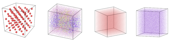
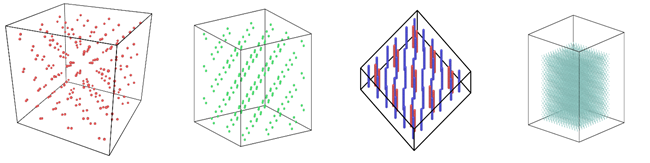
Figure 1: Image view of datasets from OVITO (scientific data visualization and analysis software for molecular and other particle-based simulation model). Images are listed in order 1a-1h, subfigure 1a- 1h represents a small portion of simulation domain for Atomic Fluid (Lennard Jones), rhodo(protein), liquid crystal(lc), copper(eam), stilliger webner(sw), Terasoff, water, polyethylene datasets respectively.
Table 1 and Figure 1 shows the image view of datasets used for the single and multi-node analysis. For visualization of all datasets was done using OVITO, scientific data visualization and analysis software for molecular and other particle-based simulation model. For single node performance study, all the datasets shown in Table 2 were used, and for multi-node study Atomic fluid was considered for benchmarking.
Performance Analyses on Single Node
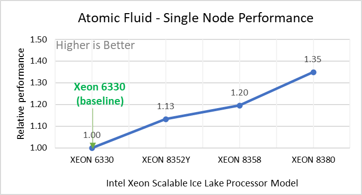
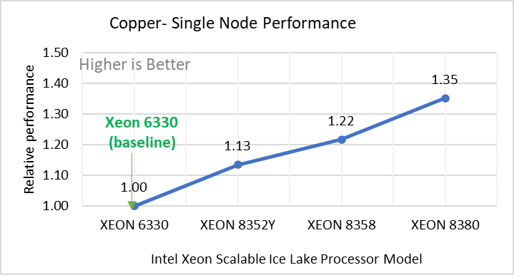
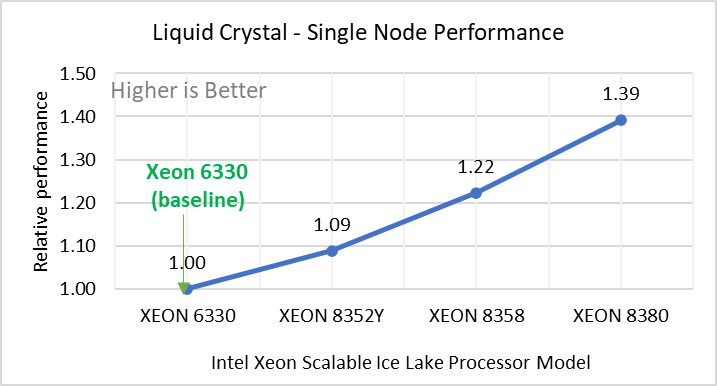
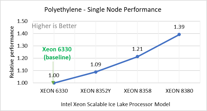
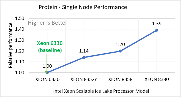
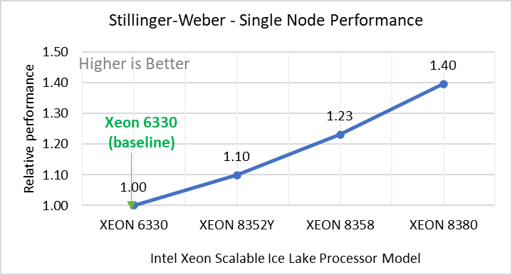
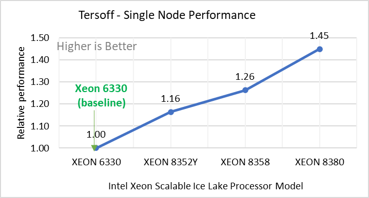
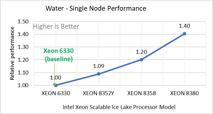
Figure 2: Single Node Performance of LAMMPS across the datasets with Intel Ice Lake processor model. Each graph in Figure 2 is an individual subfigure, labeled (a-h) in the order shown. Each subfigure (2a- 2h) represents single node performance comparison across the Xeon processors with Xeon 6330 as baseline for Atomic Fluid (Lennard Jones), rhodo(protein), liquid crystal(lc), copper(eam), stilliger webner(sw), Terasoff, water, polyethylene datasets respectively.
Figure 2 shows the single node performance for the eight datasets (sub figure 2a-h) listed in Table 2 with the four Ice Lake processor model available for evaluation of LAMMPS.
For ease of comparison across the processor model, the relative performance of the datasets has been included into a different graph. However, it is worth noting that each dataset behaves individually when performance is considered, as each uses different molecular potentials and have different number of atoms. Figure 2 shows that increases in the core count in the processor model increases the performance, across the dataset used. Next, by comparing the relative numbers to the baseline processor Xeon 6330(28C) with Xeon 8380(40C), we measured a 30 to 45 percent performance gain with these datasets. A fraction of these boosts was due to frequency of the processor model.
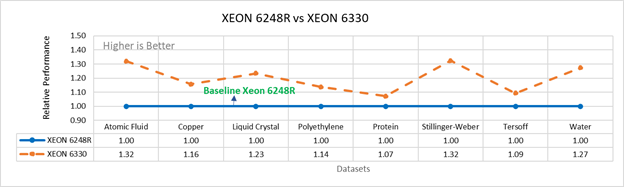
Figure 3a: Performance of LAMMPS on Cascade Lake (Xeon 6248R) in comparison to Ice Lake (Xeon 6330)
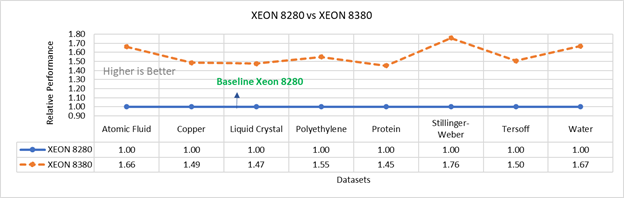
Figure 3b: Performance of LAMMPS on Cascade Lake (Xeon 8280) in comparison to Ice Lake (Xeon 8380)
Figure 3 compares the performance of the mid-bin Cascade Lake 6248R (24core) to the Ice Lake 6330 (28 core), and the top end Cascade Lake 8280 (28 core) to the Ice Lake 8380 (40 core) From the figure 3a, Ice Lake 6330 is up to 30 percent faster than the 6248R. The Xeon 6330 has 16 percent more cores, and 9 percent faster memory bandwidth. Figure 3b shows Ice Lake 8380 is up to 75 percent faster than the Xeon 8280 on single node tests, this is in line with the 42 percent additional cores and 9 percent faster memory bandwidth. These results are due to a higher processor speed wherein more data can be accessed by each core.
Performance Analysis on Multi-Node
To analyze the scalability test with strong and weak scaling, we used the Atom Fluid (LJ) dataset from the Intel package. The job run time was 7900 steps with 512000 atoms in the simulation system.
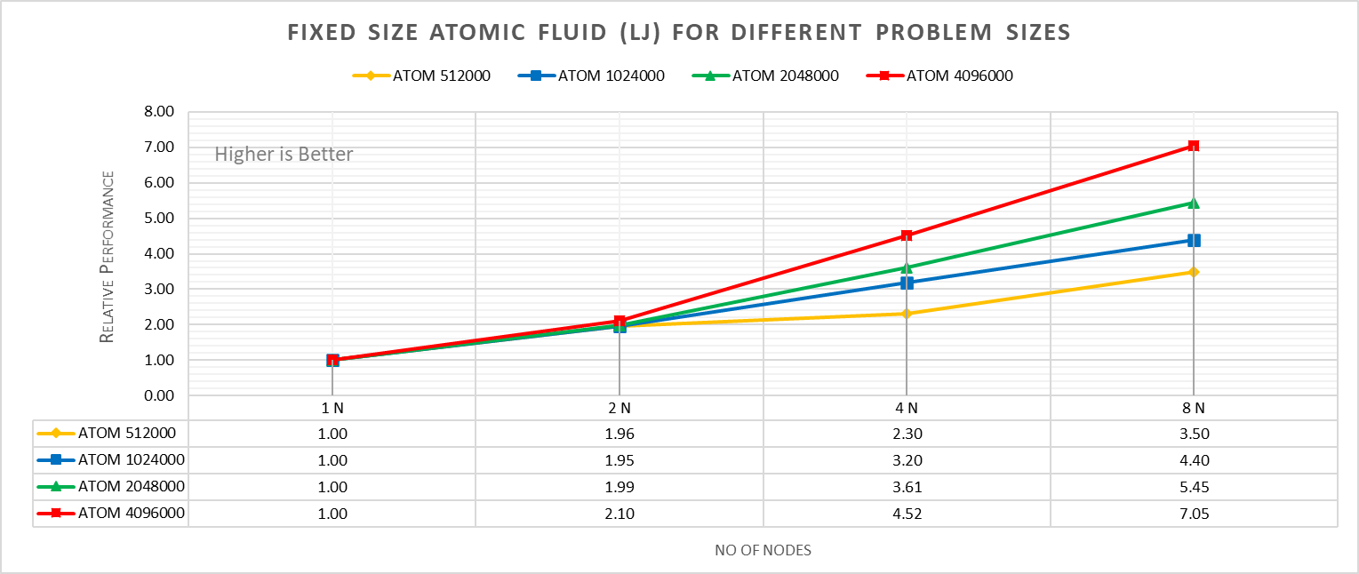
Figure 4a: Fixed size Atomic fluid (LJ) for different problem size (strong scaling) w/ Xeon 8380
With strong scaling, we referred to the fixed problem size and increasing the parallel processes (Amdahl’s law). Whereas in weak scaling, we varied the atom size from 512000 atoms to 4096000 atoms in the simulation environment with an increase in the parallel processes (Gustafson-Barsis law). The test bed included DellEMC Poweredge R750 servers each with dual Ice Lake Xeon 8380 processors an NVIDIA Networking HDR interconnect running at 200 Gbps.Figure 4a plots the fixed-size relative performance for four different problem sizes, viz, 512000,1024000,2048000, and 4096000 atoms, on different number of nodes.
The relative performance is normalized by single node performance. Hence, the single node performance for each curve is 1.00 (unity). Relative Performance for fixed size Atomic fluid was calculated by the following equation:
Relative Performance = loop time of ‘N’ node / loop time for single node
Loop time is the total wall-clock time for the simulation to run. It can be observed that relative performance increases with increase in problem size. This is because for smaller problems system spend more time in inter-nodal communications. Time spent in communication at 8 nodes is 61.91%, 59.74%,48.42%,45.04% for 512000,1024000,2048000,4096000 atom size respectively.
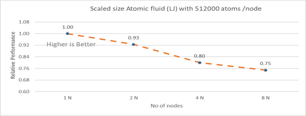
Figure 4b: Scaled size Atomic fluid (LJ) with 512000 atoms per node (weak scaling) w/ Xeon 8380
Figure 4b plots the scaled-size efficiency for runs with 512000 atoms per node. Thus, a scaled-size 2 node run is for 1024000 atoms; 8 node runs is for 4096000 atoms. Relative Performance for Scaled size Atomic fluid was calculated by the following equation:
Relative Performance= loop time for ‘n’ node/ (loop time for single node * number of nodes)
Weak scaling efficiency decreases with increase in no of nodes in the investigated range. This is due to the fact for larger number of nodes the time spend in MPI communication is larger. Time spent in communication with scaled size atom for 1N, 2N, 4N and 8 N are 27.17%, 32.42 %, 40.87%, 45.04 % respectively.
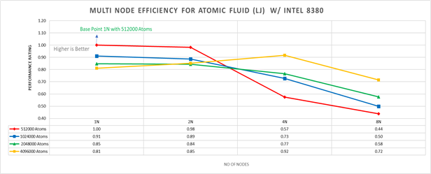
Figure 5: Multi-node efficiency for Atomic Fluid (LJ) w/ I 8380
Figure 5 plots the multi-node efficiency for Atomic Fluid with Xeon 8380. The relative performance is normalized by single node with 512000 atoms performance. Hence, the single node performance for 512000 atoms is 1.00 (unity). This point is taken as baseline for other comparison.
Performance Rating = (loop time * number of atoms)/ (loop time for 512000 atoms on 1 node * number of nodes * 512000)
We observed that for smaller systems, such as those with fewer atoms, the efficiency of strong scaling decreases as the system spends more time in MPI communication; whereas in larger systems with many atoms, the efficiency of strong scaling increases as the time spent in pair-wise force calculation becomes dominant. For weak scaling, as the no of nodes increases the efficiency of weak scaling decreases.
Conclusion
The Ice Lake processor-based Dell EMC Power Edge servers, with its hardware feature upgrades over Cascade Lake, demonstrate up to 50 to70 percent performance gain for all the datasets used for benchmarking LAMMPS. Watch our blog site for updates!