


Unisphere for PowerMax Workload Planner
Workload Planner (WLP) is a FAST component used to display performance metrics to calculate VMAX component utilizations and storage group Service Level Objective compliance. It allows for more informed workload monitoring, using up-stream components (Unisphere GUI and REST API) with respect to current VMAX performance capacity.
WLP is supported on arrays running 5977 and upwards code levels. Each service level and workload type has a response band associated with it. When a storage group (workload) is said to be compliant, it is operating within the associated response time band.
When assessing the compliance of a storage group, Workload Planner calculates its weighted response time for the past 4 hours and the past 2 weeks, and then compares the two values to the maximum response time associated with its given service level. If both calculated values fall within (under) the service level-defined response time band, the compliance state is STABLE. If one of them complies and the other is out of compliance, then the compliance state is MARGINAL. If both are out of compliance, then the compliance state is CRITICAL.
SG SLO compliance
To begin, let’s examine our SG SLO compliance to examine how our SG’s have been performing.
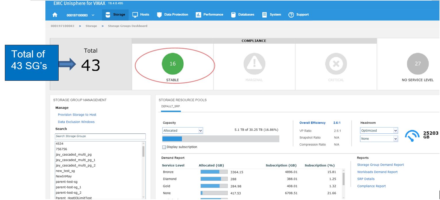 Figure 1. Storage group view
In this example, we have a total of 43 SGs with none being in a marginal or critical state. Let’s click on 16 stable SG’s and review further.
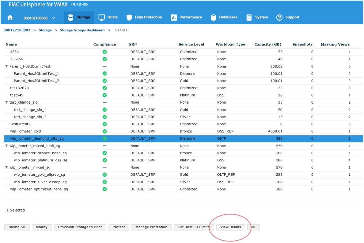
Figure 2. Storage groups drill down view
Here, we have a SG list for the array. In the second column, we see that our sg wlp_iometer_diamond is in a compliant SLO state. Let’s review this SG further by selecting this SG, and then clicking on View Details. This takes us to Details view where we can review the properties of the SG and check its performance on the right-hand side. Here, we want to select Compliance and select the storage tab.
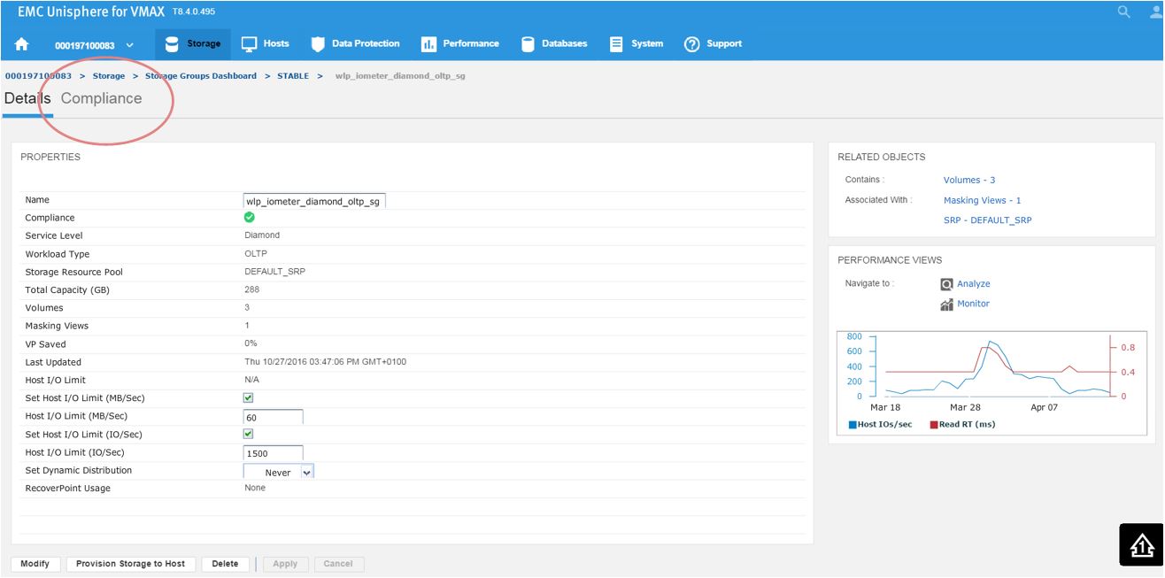
Figure 3. Storage group Details view
Here, we get greater detail on the current compliance state of the SG. We can see that it has a Diamond SLO which is stable. Currently, its capacity trend is flat, however we can also see how our response times over the windows of time. Additionally, we can review how the SG is performing compared to when it was first created.
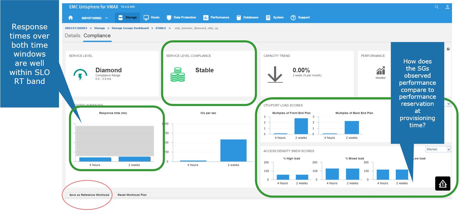
Figure 4. Storage group Compliance view
Saving a favorite reference workload
Here, we also have the ability to save this as a reference workload. For example, this SG is being used for an Oracle database, and we are happy with its performance and configuration since we rolled the application out into production.
Let’s leverage Unisphere to keep this workload for use in the future.
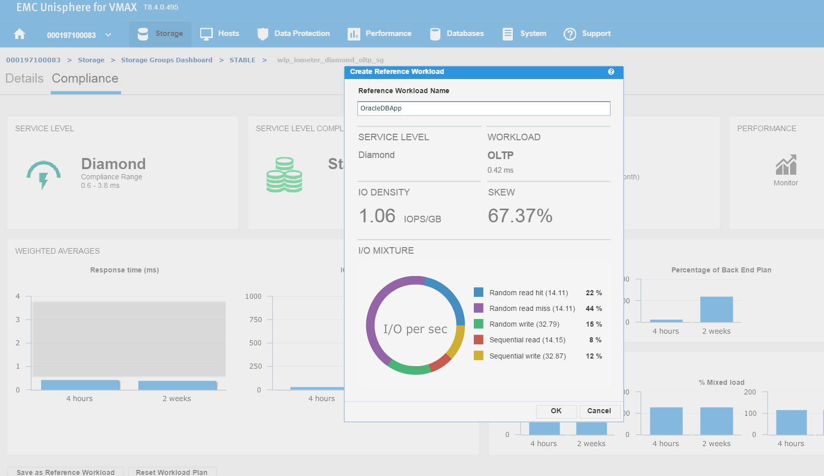
Figure 5. Create reference workload
We have named the workload OracleDBApp, so we can use this as a reference point when we roll out a similar Oracle Application with the breakdown of read and writes in terms of I/O.
Continuing along, let’s first verify that our workload type was saved correctly. To do this, go to Storage > Service Level, and select the Workload Types tab.
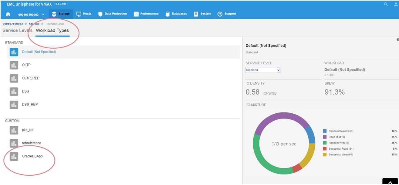
Figure 6. Save workload type
Now, we can see the reference workload we have customized in OracleDBApp. Since we are satisfied with the configuration of this application’s performance, we can leverage this workload type for use in the future when rolling out similar type applications.
Let’s see how we can use this in the provisioning wizard.
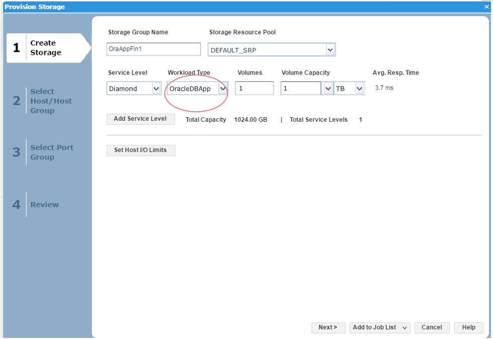
Figure 7. Create storage group view
Here, we can see that as we have received another request from our finance team for a new SG, so we decide to choose the workload type we had previously customized as a reference point and use this for the new SG.
Investigating an SG compliance issue with WLP
Let’s begin with a realistic scenario. One of our application teams contacted us over an issue with an SG, and they wanted us to investigate further to see if it has had any compliance issues in the recent past. Let’s begin with looking at the SG compliance report.
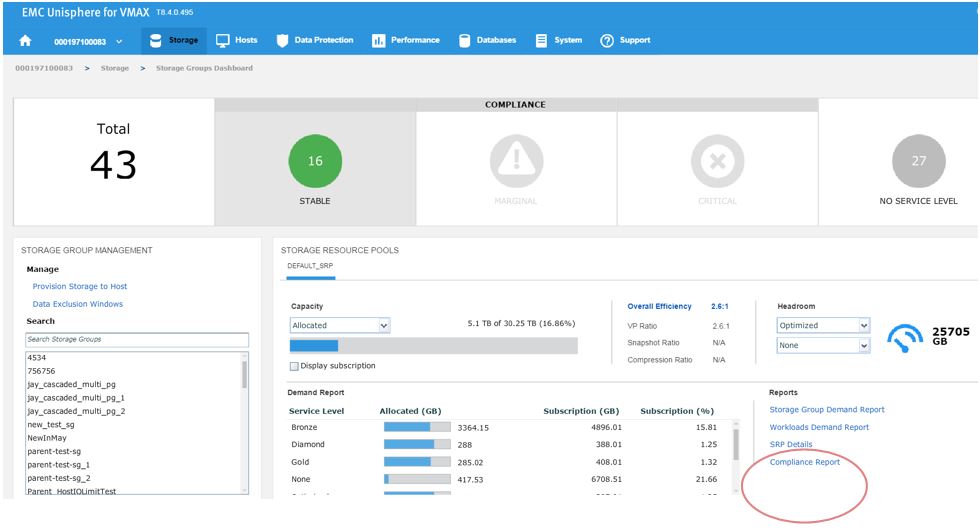
Figure 8. Storage group compliance view 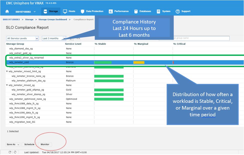
Figure 9. Storage group compliance issue
Here we see for the SG wlp_iometer_cold, we had a compliance issue in the last 3 months, with some being in a marginal state and some being in a critical state. If we select the SG, we have the option of saving the report off for reference or to potentially show to the application owner. We can also select Monitor, which will launch us directly into the Performance section of Unisphere shown in the following figure where we can check specific metrics.
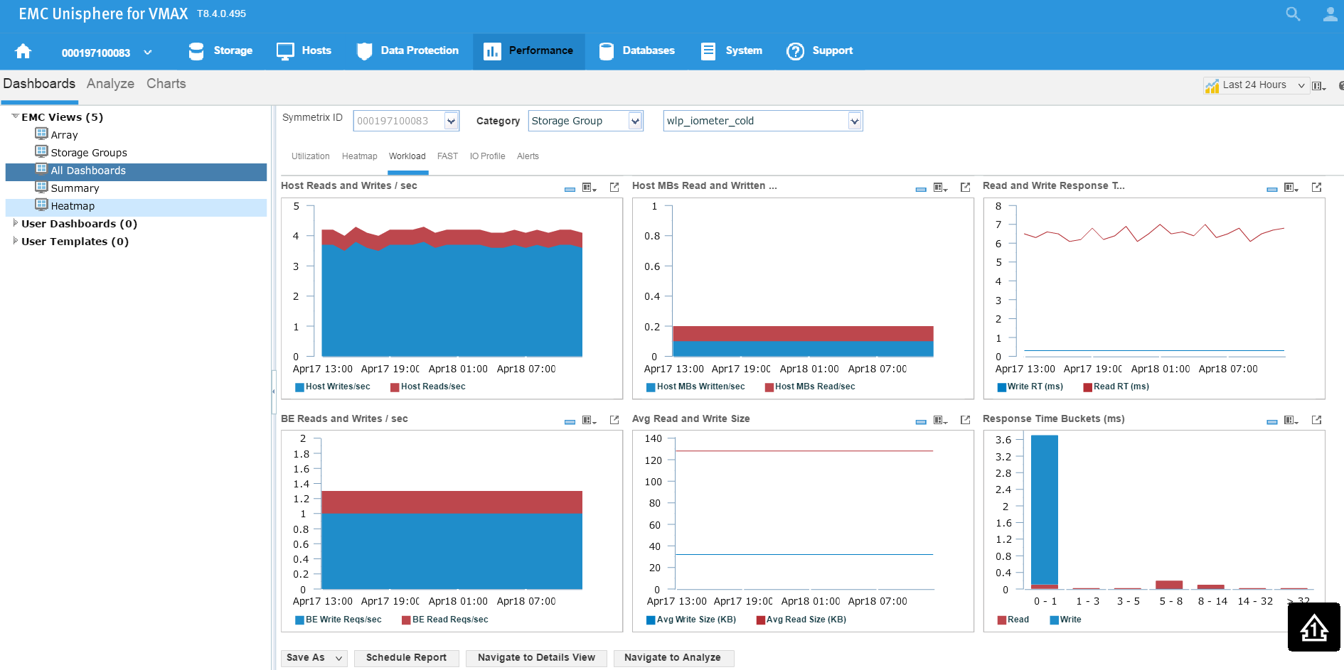
Figure 10. Storage group performance view
Examining headroom for Service Level and Workload Type combinations
In this section, I will be covering how to examine the available headroom for various Service Level and Workload Type combinations. Also, I will show you how to run a suitability check while provisioning more storage to an existing storage group.
The headroom available shows the space available for a certain combination of service level and workload type if all the remaining capacity was on that type. Here, I wanted to show you two examples for different service levels to showcase the calculation change.
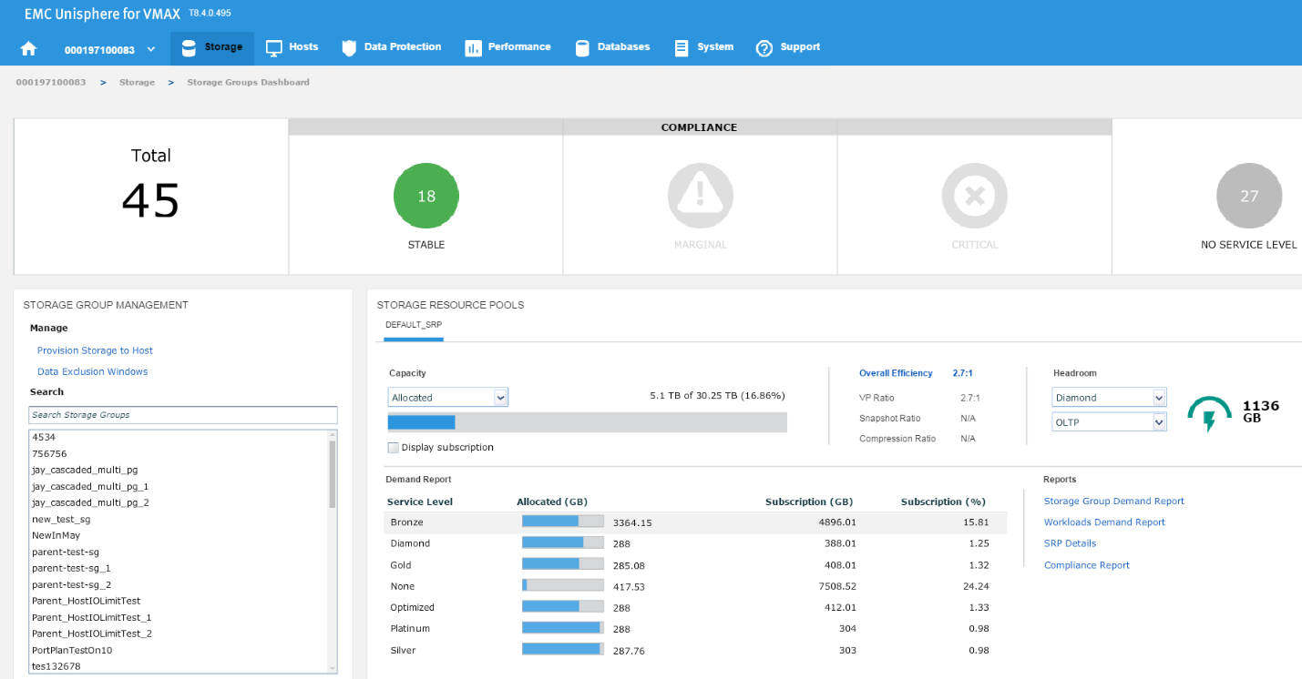
Figure 11. Storage group compliance view
In this example, we have chosen a Diamond SLO and an OLTP workload, which allows us free space of 1136 GB with that combination for that array. Let’s change the parameters, and see what happens.
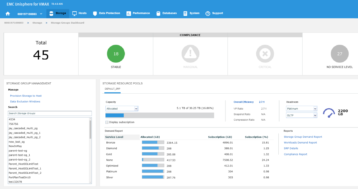
Figure 12. Storage group resource pools view
Now, we have 2200 GB of space available at a platinum level, which is almost double the capacity we had at Diamond level. These can be useful indicators of when we have an array that is nearing capacity as we can gauge which of our most important applications can go on to which SLO so we can maximize the efficiency of our storage.
Expanding the capacity of an existing SG
Now, let’s examine how we can expand the capacity of an existing SG while checking its suitability through the provisioning wizard. Let’s start at the SG list view in the storage group dashboard. We select our SG and then click on View Details.
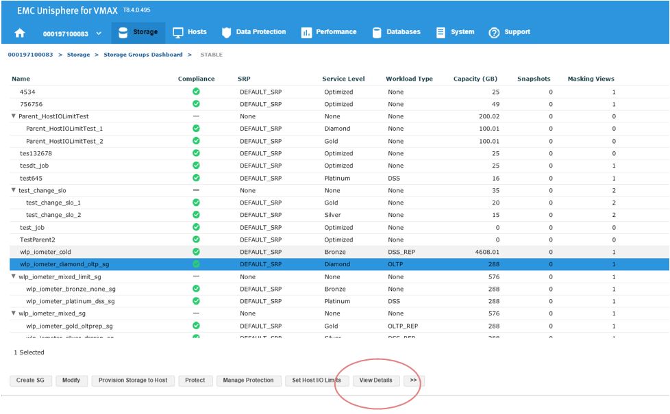
Figure 13. Storage group dashboard view
This will take us to the Details view of the wlp_iometer_diamond SG, which is the SG we want to expand. We then select Modify to start the process.
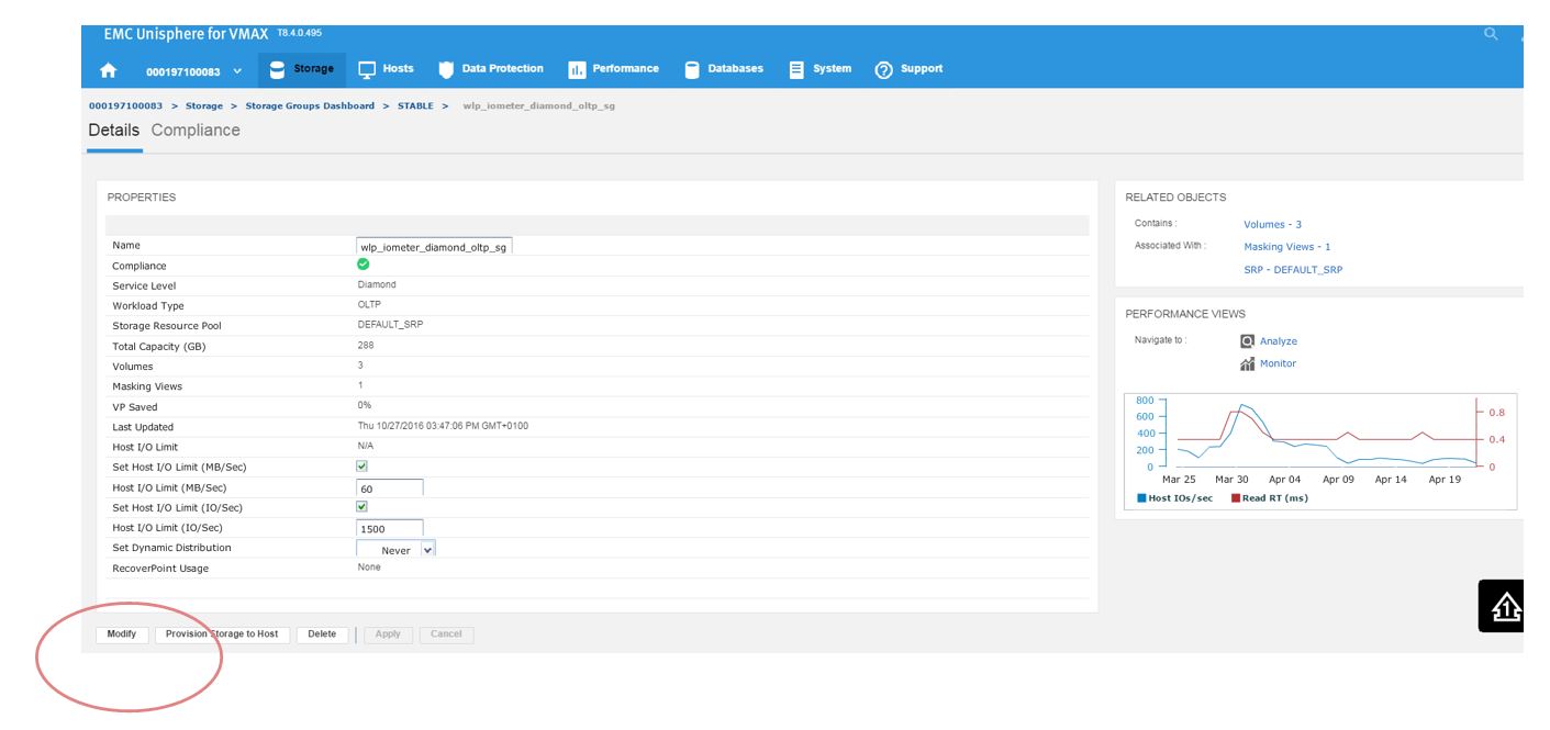
Figure 14. Storage group properties view
This launches the Modify Storage Group wizard shown in the following figure. We have received a request from the application owner that they need additional storage, however we wanted to be sure prior to allocation that they will not breach their SLO compliance nor experience any performance problems.
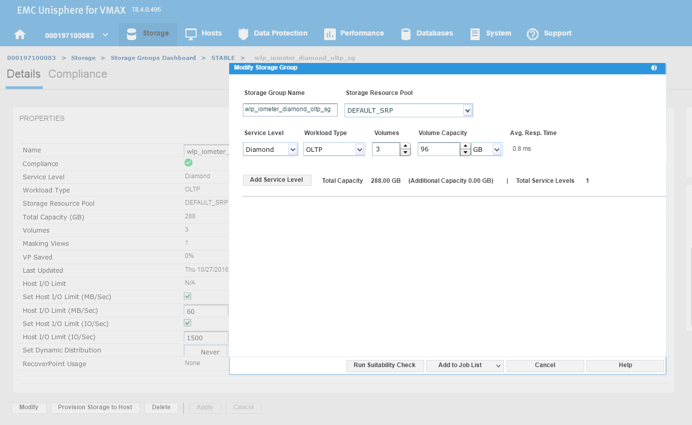
Figure 15. Modify storage group view
We have agreed with the application owners to grant them an additional 96 GB of storage, which will expand their capacity by roughly 25%. This allows us to increase the number of volumes by 1, and then select Run Suitability Check to verify this change won’t affect the performance of the SG adversely.
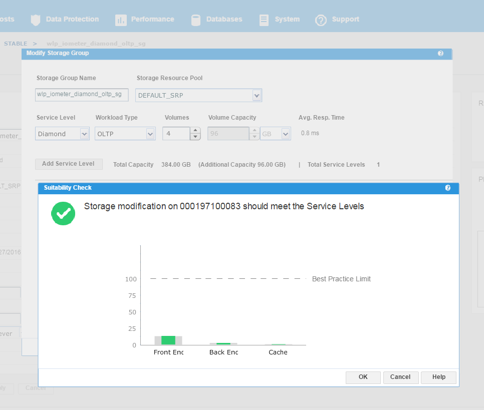
Figure 16. Storage group service levels view
We can see that the check has completed successfully and that increasing the capacity of the SG will not have any adverse effects on its performance. This promotes good housekeeping in terms of the storage array as we prevent poor configurations from being rolled out. At this stage, we can select Run Now and add to the job list to run later.
Data Exclusion Windows
In this section, I will be covering how to manage Data Exclusion Windows. This procedure explains how to manage Data Exclusion windows for calculating headroom and suitability.
Peaks in storage system statistics can occur due to:
- Anomalies or unusual events
- Recurring maintenance during off-hours that fully loads the storage system
Due to the way this data is condensed and used, unexpected headroom and suitability results can occur. There are two ways to improve the handling of these cases:
- One-time exclusion period – When the one-time exclusion period value is set, all statistics before this time are ignored. This helps resolve anomalies or unusual events where a significant one-time peak distorts the results due to reliance on two weeks of data points. This is set system wide for all components.
- Recurring exclusion period – You can select n of 42 buckets to use in admissibility checks. This is set system wide for all components. Recurring exclusion periods are repeating periods of selected weekday or time slot combinations where collected data is ignored for the purpose of compliance and admissibility considerations. The data is still collected and reported, but it is not used in those calculations.
Let’s begin at our usual starting point, the storage group dashboard, by selecting the Data Exclusion Window.
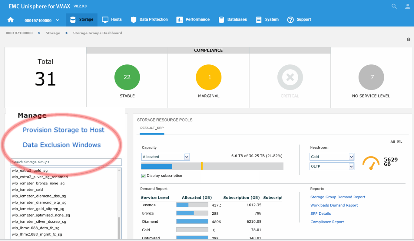
Figure 17. Data Exclusion Windows
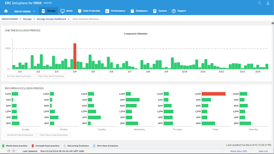
Figure 18. Data Exclusion Windows
All the component utilizations for the prior two-week period are compared, and the greatest (with respect to its individual best-practice limit) is displayed across the top of this display. Each weekly time period, represented by two bars in the top display, is also displayed across the bottom.
Now we will set a one-time exclusion window. When you click on the tallest bar in the top display, all history up to that time is shaded. You can then select Set One-time Exclusion so the bottom display panel is recalculated excluding that time frame.
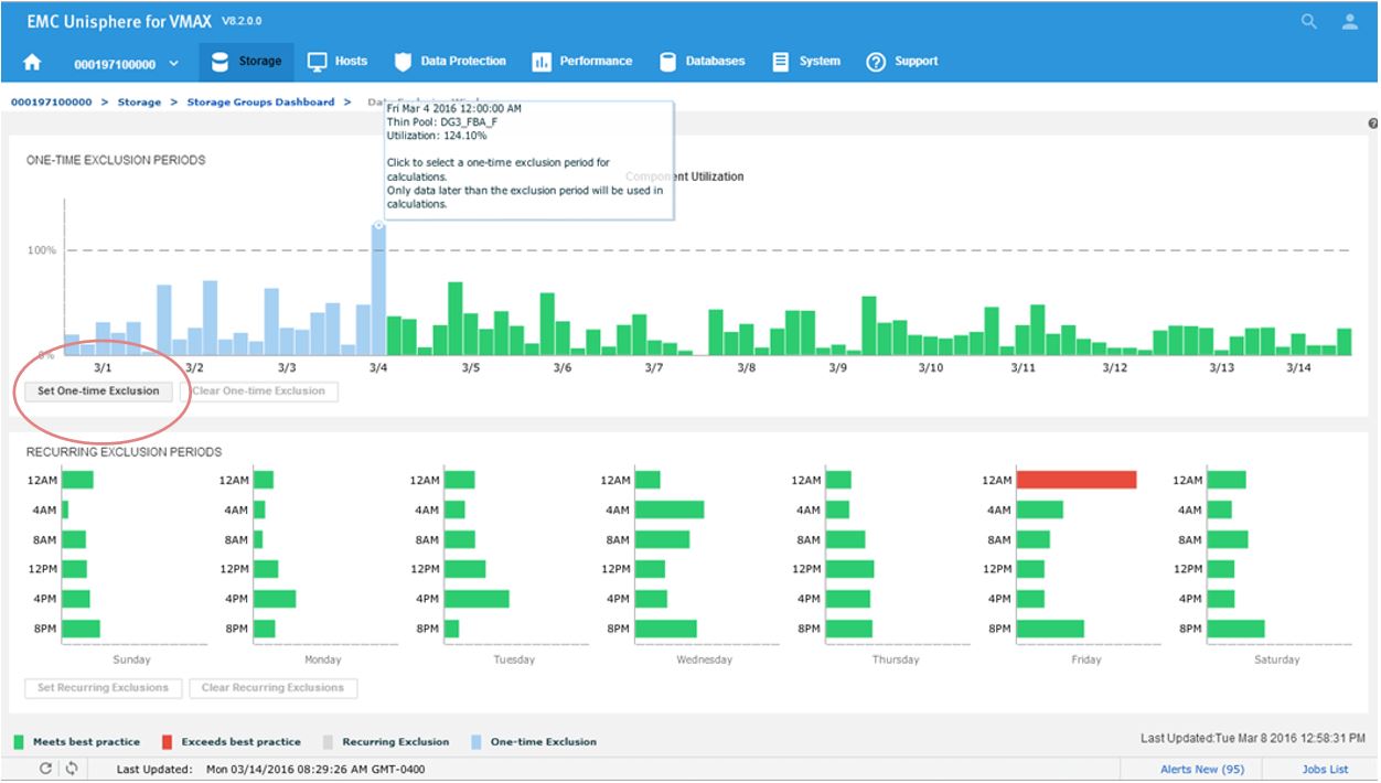
Figure 19. Data Exclusion time window view
After setting the exclusion, you can now see that at 12 a.m, we are green in the bottom panel as we have chosen to ignore that specific timeframe in our calculations.
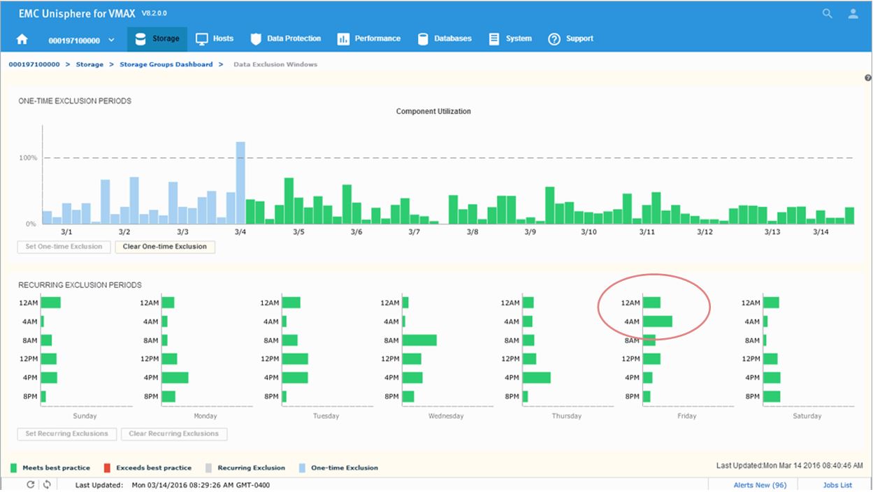
Figure 20. Data Exclusion Windows time view
Next, we will look to set a recurring Exclusion window:
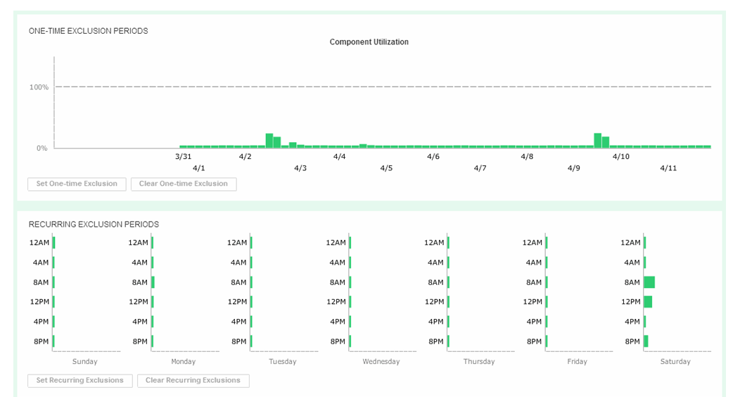
Figure 21. Set recurring Data Exclusion Window
If you click on the bars in the bottom display, their state will toggle, shading themselves and the two corresponding bars in the top display to set any weekly period to be excluded from all suitability and headroom calculations from there on for the future.
FAST Array Advisor
In this section, I will be covering how to leverage FAST Array Advisor to see if you could move workloads between arrays. The FAST Array Advisor wizard determines the performance impact of migrating the workload from one storage system (source) to another storage system (target). If the wizard determines that the target storage system can absorb the added workload, it automatically creates all the necessary auto provisioning groups to duplicate the source workload on the target system.
Let’s pick a suitable SG PF_NDM_2_SG and select the More Options button.
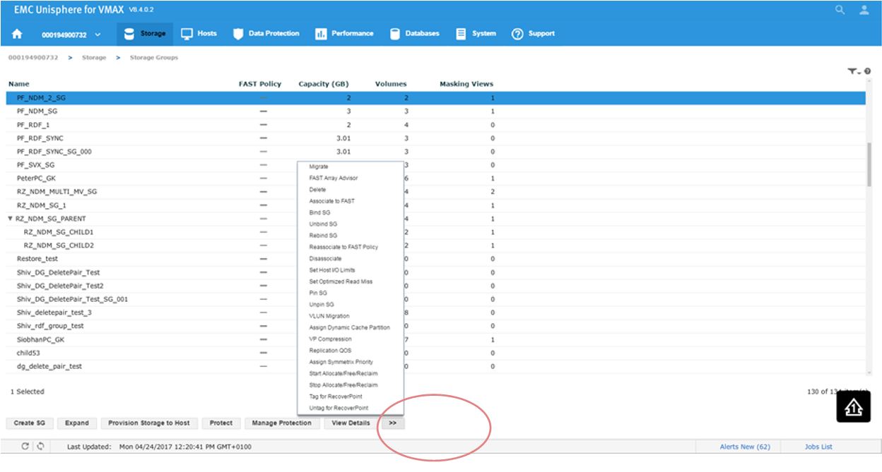
Figure 22. Storage group selection view
This will present us with a series of options. Second from the top, we see FAST Array Advisor, so we select that.
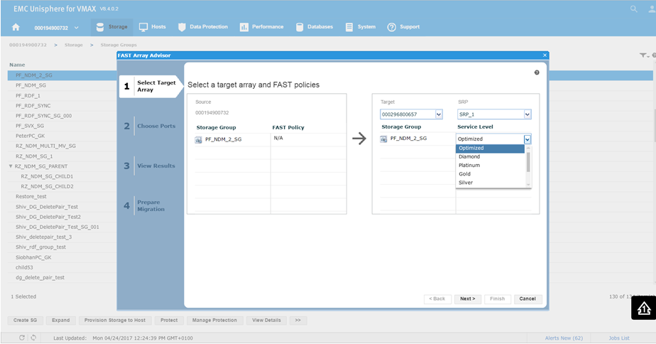
Figure 23. Select target array view
This will bring us the wizard where we select the source and target array. In this example, 0732 is a V1 running 76 code, and we want to look at the possibility of moving it to 0657 which is a V3 running 77 codes. This is viewed in terms of a migration of the SG off the older source array and on the newer target array. You can see that on a V1, we did not have service levels, however we can set them on our V3 array. For this example, we choose a Silver SLO and click Next.
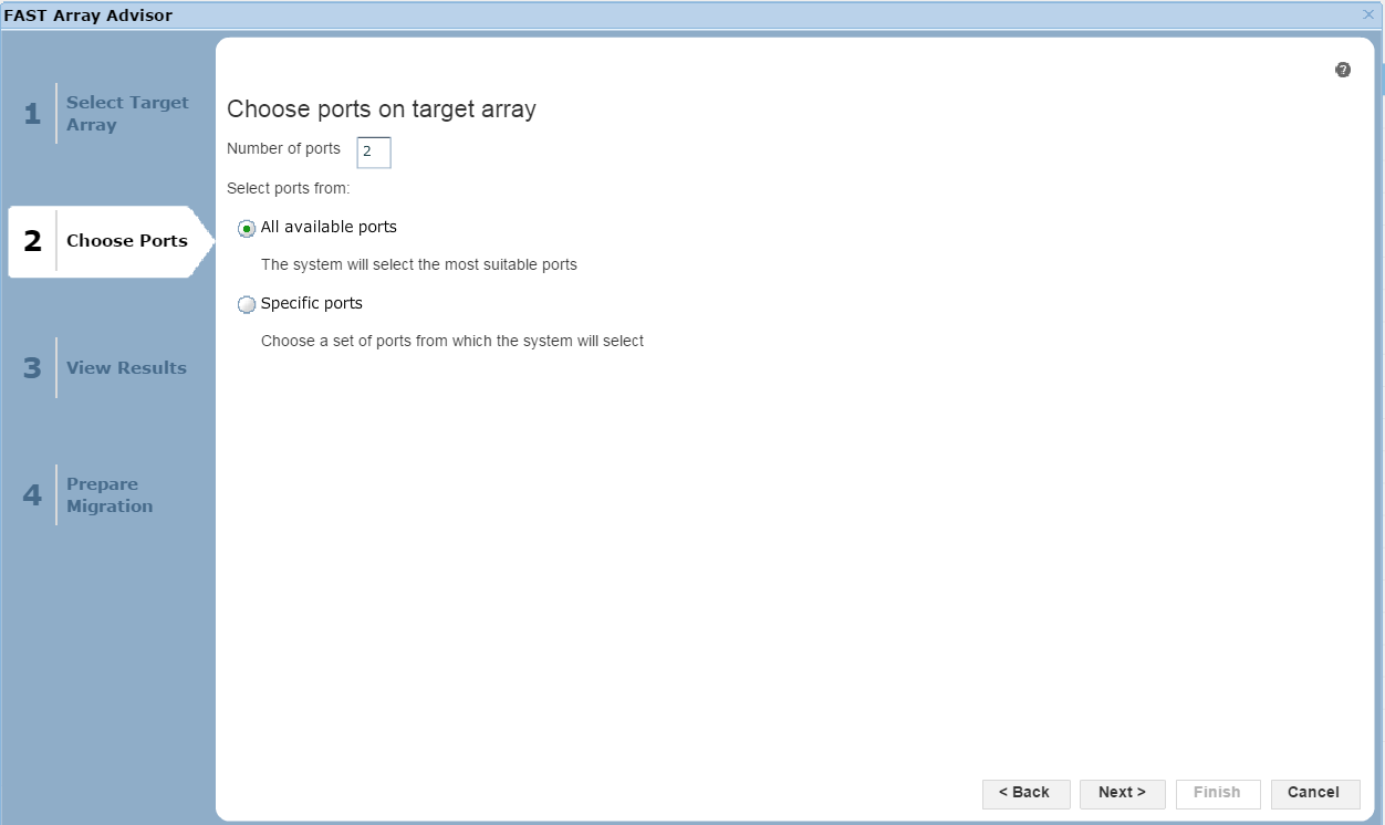
Figure 24. Port selection view
In this section of the wizard, we have the option of allowing Unisphere to choose the most suitable ports based on how busy they are, or we can select specific ports if we like. Click Next to view the results.
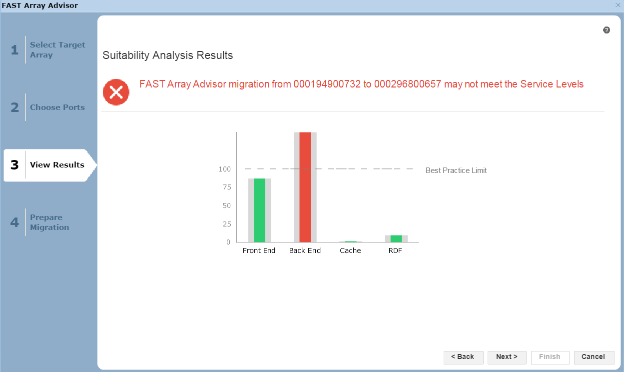
Figure 25. Suitability analysis view
Here, we see the results of the potential migration. The front end, the cache utilization, and the RDF impact all look fine. That said, in the back end, we would exceed our Best Practice Limit, so we may suffer from contention and performance issues as a result. It would be up to the individual customer to proceed in these circumstances, however we would recommend adhering to best practices. In this case, let’s select Next to view the final screen of the wizard.
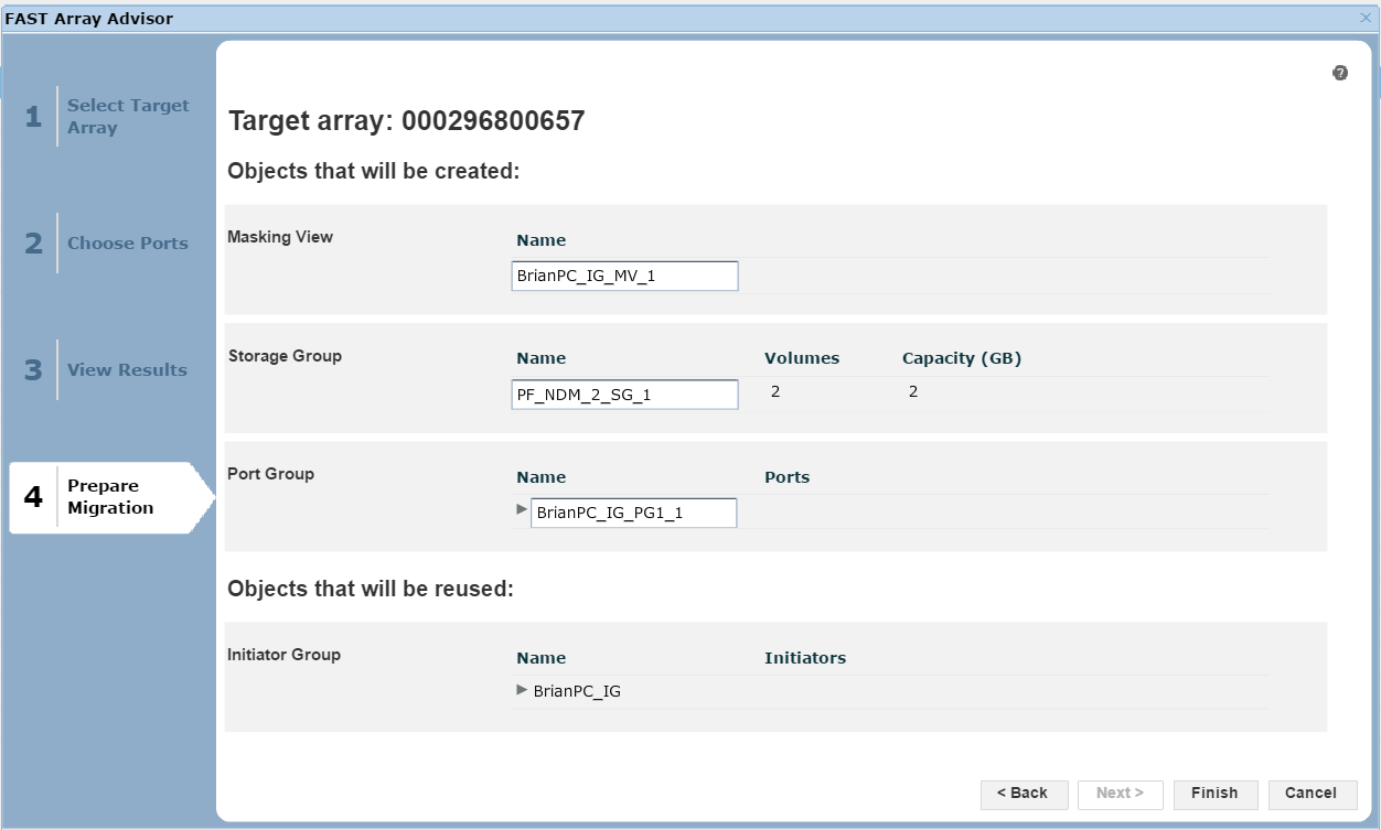
Figure 26. Prepare migration view
Here, we are presented with a summary of the migration if we were to go ahead, listing what objects, such as the masking views, storage groups and port groups, would be created on the target array 0657. At this point, we can click Finish to begin the migration.
Author: Finbarr O’Riordan, ISG Technical Program Manager for Transformation