


Training Neural Network Models for Financial Services with Intel® Xeon Processors
Fri, 12 Jun 2020 12:22:20 -0000
|Read Time: 0 minutes
Originally published on Nov 5, 2018 9:10:17 AM
Time series is a very important type of data in the financial services industry. Interest rates, stock prices, exchange rates, and option prices are good examples for this type of data. Time series forecasting plays a critical role when financial institutions design investment strategies and make decisions. Traditionally, statistical models such as SMA (simple moving average), SES (simple exponential smoothing), and ARIMA (autoregressive integrated moving average) are widely used to perform time series forecasting tasks.
Neural networks are promising alternatives, as they are more robust for such regression problems due to flexibility in model architectures (e.g., there are many hyperparameters that we can tune, such as number of layers, number of neurons, learning rate, etc.). Recently applications of neural network models in the time series forecasting area have been gaining more and more attention from statistical and data science communities.
In this blog, we will firstly discuss about some basic properties that a machine learning model must have to perform financial service tasks. Then we will design our model based on these requirements and show how to train the model in parallel on HPC cluster with Intel® Xeon processors.
Requirements from Financial Institutions
High-accuracy and low-latency are two import properties that financial service institutions expect from a quality time series forecasting model.
High Accuracy A high level of accuracy in the forecasting model helps companies lower the risk of losing money in investments. Neural networks are believed to be good at capturing the dynamics in time series and hence yield more accurate predictions. There are many hyperparameters in the model so that data scientists and quantitative researchers can tune them to obtain the optimal model. Moreover, data science community believes that ensemble learning tends to improve prediction accuracy significantly. The flexibility of model architecture provides us a good variety of model members for ensemble learning.
Low Latency Operations in financial services are time-sensitive. For example, high frequency trading usually requires models to finish training and prediction within very short time periods. For deep neural network models, low latency can be guaranteed by distributed training with Horovod or distributed TensorFlow. Intel® Xeon multi-core processors, coupled with Intel’s MKL optimized TensorFlow, prove to be a good infrastructure option for such distributed training.
With these requirements in mind, we propose an ensemble learning model as in Figure 1, which is a combination of MLP (Multi-Layer Perceptron), CNN (Convolutional Neural Network) and LSTM (Long Short-Term Memory) models. Because architecture topologies for MLP, CNN and LSTM are quite different, the ensemble model has a good variety in members, which helps reduce risk of overfitting and produces more reliable predictions. The member models are trained at the same time over multiple nodes with Intel® Xeon processors. If more models need to be integrated, we just add more nodes into the system so that the overall training time stays short. With neural network models and HPC power of the Intel® Xeon processors, this system meets the requirements from financial service institutions.
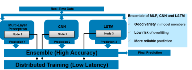 Training high accuracy ensemble model on HPC cluster with Intel® Xeon processors
Fast Training with Intel® Xeon Scalable Processors
Our tests used Dell EMC’s Zenith supercomputer which consists of 422 Dell EMC PowerEdge C6420 nodes, each with 2 Intel® Xeon Scalable Gold 6148 processors. Figure 2 shows an example of time-to-train for training MLP, CNN and LSTM models with different numbers of processes. The data set used is the 10-Year Treasury Inflation-Indexed Security data. For this example, running distributed training with 40 processes is the most efficient, primarily due to the data size in this time series is small and the neural network models we used did not have many layers. With this setting, model training can finish within 10 seconds, much faster than training the models with one processor that has only a few cores, which typically takes more than one minute. Regarding accuracy, the ensemble model can predict this interest rate with MAE (mean absolute error) less than 0.0005. Typical values for this interest rate is around 0.01, so the relative error is less than 5%.
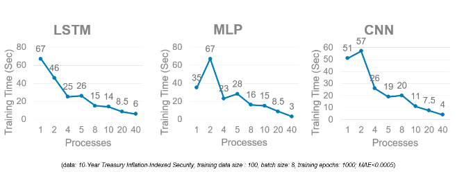 Training time comparison: Each of the models is trained on a single Dell EMC PowerEdge C6420 with 2x Intel Xeon® Scalable 6148 processors
Conclusion
With both high-accuracy and low-latency being very critical for time series forecasting in financial services, neural network models trained in parallel using Intel® Xeon Scalable processors stand out as very promising options for financial institutions. And as financial institutions need to train more complicated models to forecast many time series with high accuracy at the same time, the need for parallel processing will only grow.
Related Blog Posts
Optimizing AI: Meeting Unstructured Storage Demands Efficiently

Thu, 21 Mar 2024 14:46:23 -0000
|Read Time: 0 minutes
The surge in artificial intelligence (AI) and machine learning (ML) technologies has sparked a revolution across industries, pushing the boundaries of what's possible. However, this innovation comes with its own set of challenges, particularly when it comes to storage. The heart of AI's potential lies in its ability to process and learn from vast amounts of data, most of which is unstructured. This has placed unprecedented demands on storage solutions, becoming a critical bottleneck for advancing AI technologies.
Navigating the complex landscape of unstructured data storage is no small feat. Traditional storage systems struggle to keep up with the scale and flexibility required by AI workloads. Enterprises find themselves at a crossroads, seeking solutions that can provide scalable, affordable, and fault-tolerant storage. The quest for such a platform is not just about meeting current needs but also paving the way for the future of AI-driven innovation.
The current state of ML and AI
The evolution of ML and AI technologies has reshaped industries far and wide, setting new expectations for data processing and analysis capabilities. These advancements are directly tied to an organization's capacity to handle vast volumes of unstructured data, a domain where traditional storage solutions are being outpaced.
ML and AI applications demand unprecedented levels of data ingestion and computational power, necessitating scalable and flexible storage solutions. Traditional storage systems—while useful for conventional data storage needs—grapple with scalability issues, particularly when faced with the immense file quantities AI and ML workloads generate.
Although traditional object storage methods are capable of managing data as objects within a pool, they fall short when meeting the agility and accessibility requirements essential for AI and ML processes. These storage models struggle with scalability and facilitating the rapid access and processing of data crucial for deep learning and AI algorithms.
The dire necessity of a new kind of storage solution is evident as the current infrastructure is unable to cope with the silos of unstructured data. These silos make it challenging to access, process, and unify data sources, which in turn cripples the effectiveness of AI and ML projects. Furthermore, the maximum storage capacity of traditional storage, tethering at tens of terabytes, is insufficient for the needs of AI-driven initiatives which often require petabytes of data to train sophisticated models.
As ML and AI continue to advance, the quest for a storage solution that can support the growing demands of these technologies remains pivotal. The industry is in dire need of systems that provide ample storage and ensure the flexibility, reliability, and performance efficiency necessary to propel AI and ML into their next phase of innovation.
Understanding unstructured storage demands for AI
The advent of AI and ML has brought unprecedented advancements across industries, enhancing efficiency, accuracy, and the ability to manage and process large datasets. However, the core of these technologies relies on the capability to store, access, and analyze unstructured data efficiently. Understanding the storage demands essential for AI applications is crucial for businesses looking to harness the full power of AI technology.
High throughput and low latency
For AI and ML applications, time is of the essence. The ability to process data at high speeds with high throughput and access it with minimal delay and low latency are non-negotiable requirements. These applications often involve complex computations performed on vast datasets, necessitating quick access to data to maintain a seamless process. For instance, in real-time AI applications such as voice recognition or instant fraud detection, any delay in data processing can critically impact performance and accuracy. Therefore, storage solutions must be designed to accommodate these needs, delivering data as swiftly as possible to the application layer.
Scalability and flexibility
As AI models evolve and the volume of data increases, the need for scalability in storage solutions becomes paramount. The storage architecture must accommodate growth without compromising on performance or efficiency. This is where the flexibility of the storage solutions comes into play. An ideal storage system for AI would scale in capacity and performance, adapting to the changing demands of AI applications over time. Combining the best of on-premises and cloud storage, hybrid storage solutions offer a viable path to achieving this scalability and flexibility. They enable businesses to leverage the high performance of on-premise solutions and the scalability and cost-efficiency of cloud storage, ensuring the storage infrastructure can grow with the AI application needs.
Data durability and availability
Ensuring the durability and availability of data is critical for AI systems. Data is the backbone of any AI application, and its loss or unavailability can lead to significant setbacks in development and performance. Storage solutions must, therefore, provide robust data protection mechanisms and redundancies to safeguard against data loss. Additionally, high availability is essential to ensure that data is always accessible when needed, particularly for AI applications that require continuous operation. Implementing a storage system with built-in redundancy, failover capabilities, and disaster recovery plans is essential to maintain continuous data availability and integrity.
In the context of AI where data is continually ingested, processed, and analyzed, the demands on storage solutions are unique and challenging. Key considerations include maintaining high throughput and low latency for real-time processing, establishing scalability and flexibility to adapt to growing data volumes, and ensuring data durability and availability to support continuous operation. Addressing these demands is critical for businesses aiming to leverage AI technologies effectively, paving the way for innovation and success in the digital era.
What needs to be stored for AI?
The evolution of AI and its underlying models depends significantly on various types of data and artifacts generated and used throughout its lifecycle. Understanding what needs to be stored is crucial for ensuring the efficiency and effectiveness of AI applications.
Raw data
Raw data forms the foundation of AI training. It's the unmodified, unprocessed information gathered from diverse sources. For AI models, this data can be in the form of text, images, audio, video, or sensor readings. Storing vast amounts of raw data is essential as it provides the primary material for model training and the initial step toward generating actionable insights.
Preprocessed data
Once raw data is collected, it undergoes preprocessing to transform it into a more suitable format for training AI models. This process includes cleaning, normalization, and transformation. As a refined version of raw data, preprocessed data needs to be stored efficiently to streamline further processing steps, saving time and computational resources.
Training datasets
Training datasets are a selection of preprocessed data used to teach AI models how to make predictions or perform tasks. These datasets must be diverse and comprehensive, representing real-world scenarios accurately. Storing these datasets allows AI models to learn and adapt to the complexities of the tasks they are designed to perform.
Validation and test datasets
Validation and test datasets are critical for evaluating an AI model's performance. These datasets are separate from the training data and are used to tune the model's parameters and test its generalizability to new, unseen data. Proper storage of these datasets ensures that models are both accurate and reliable.
Model parameters and weights
An AI model learns to make decisions through its parameters and weights. These elements are fine-tuned during training and crucial for the model's decision-making processes. Storing these parameters and weights allows models to be reused, updated, or refined without retraining from scratch.
Model architecture
The architecture of an AI model defines its structure, including the arrangement of layers and the connections between them. Storing the model architecture is essential for understanding how the model processes data and for replicating or scaling the model in future projects.
Hyperparameters
Hyperparameters are the configuration settings used to optimize model performance. Unlike parameters, hyperparameters are not learned from the data but set prior to the training process. Storing hyperparameter values is necessary for model replication and comparison of model performance across different configurations.
Feature engineering artifacts
Feature engineering involves creating new input features from the existing data to improve model performance. The artifacts from this process, including the newly created features and the logic used to generate them, need to be stored. This ensures consistency and reproducibility in model training and deployment.
Results and metrics
The results and metrics obtained from model training, validation, and testing provide insights into model performance and effectiveness. Storing these results allows for continuous monitoring, comparison, and improvement of AI models over time.
Inference data
Inference data refers to new, unseen data that the model processes to make predictions or decisions after training. Storing inference data is key for analyzing the model's real-world application and performance and making necessary adjustments based on feedback.
Embeddings
Embeddings are dense representations of high-dimensional data in lower-dimensional spaces. They play a crucial role in processing textual data, images, and more. Storing embeddings allows for more efficient computation and retrieval of similar items, enhancing model performance in recommendation systems and natural language processing tasks.
Code and scripts
The code and scripts used to create, train, and deploy AI models are essential for understanding and replicating the entire AI process. Storing this information ensures that models can be retrained, refined, or debugged as necessary.
Documentation and metadata
Documentation and metadata provide context, guidelines, and specifics about the AI model, including its purpose, design decisions, and operating conditions. Proper storage of this information supports ethical AI practices, model interpretability, and compliance with regulatory standards.
Challenges of unstructured data in AI
In the realm of AI, handling unstructured data presents a unique set of challenges that must be navigated carefully to harness its full potential. As AI systems strive to mimic human understanding, they face the intricate task of processing and deriving meaningful insights from data that lacks a predefined format. This section delves into the core challenges associated with unstructured data in AI, primarily focusing on data variety, volume, and velocity.
Data variety
Data variety refers to the myriad types of unstructured data that AI systems are expected to process, ranging from texts and emails to images, videos, and audio files. Each data type possesses its unique characteristics and demands specific preprocessing techniques to be effectively analyzed by AI models.
- Richer Insights but Complicated Processing: While the diverse data types can provide richer insights and enhance model accuracy, they significantly complicate the data preprocessing phase. AI tools must be equipped with sophisticated algorithms to identify, interpret, and normalize various data formats.
- Innovative AI Applications: The advantage of mastering data variety lies in the development of innovative AI applications. By handling unstructured data from different domains, AI can contribute to advancements in natural language processing, computer vision, and beyond.
Data volume
The sheer volume of unstructured data generated daily is staggering. As digital interactions increase, so does the amount of data that AI systems need to analyze.
- Scalability Challenges: The exponential growth in data volume poses scalability challenges for AI systems. Storage solutions must not only accommodate current data needs but also be flexible enough to scale with future demands.
- Efficient Data Processing: AI must leverage parallel processing and cloud storage options to keep up with the volume. Systems designed for high-throughput data analysis enable quicker insights, which are essential for timely decision-making and maintaining relevance in a rapidly evolving digital landscape.
Data velocity
Data velocity refers to the speed at which new data is generated and the pace at which it needs to be processed to remain actionable. In the age of real-time analytics and instant customer feedback, high data velocity is both an opportunity and a challenge for AI.
- Real-Time Processing Needs: AI systems are increasingly required to process information in real-time or near-real-time to provide timely insights. This necessitates robust computational infrastructure and efficient data streaming technologies.
- Constant Adaptation: The dynamic nature of unstructured data, coupled with its high velocity, demands that AI systems constantly adapt and learn from new information. Maintaining accuracy and relevance in fast-moving data environments is critical for effective AI performance.
In addressing these challenges, AI and ML technologies are continually evolving, developing more sophisticated systems capable of handling the complexity of unstructured data. The key to unlocking the value hidden within this data lies in innovative approaches to data management where flexibility, scalability, and speed are paramount.
Strategies to manage unstructured data in AI
The explosion of unstructured data poses unique challenges for AI applications. Organizations must adopt effective data management strategies to harness the full potential of AI technologies. In this section, we delve into key strategies like data classification and tagging and the use of PowerScale clusters to efficiently manage unstructured data in AI.
Data classification and tagging
Data classification and tagging are foundational steps in organizing unstructured data and making it more accessible for AI applications. This process involves identifying the content and context of data and assigning relevant tags or labels, which is crucial for enhancing data discoverability and usability in AI systems.
- Automated tagging tools can significantly reduce the manual effort required to label data, employing AI algorithms to understand the content and context automatically.
- Custom metadata tags allow for the creation of a rich set of file classification information. This not only aids in the classification phase but also simplifies later iterations and workflow automation.
- Effective data classification enhances data security by accurately categorizing sensitive or regulated information, enabling compliance with data protection regulations.
Implementing these strategies for managing unstructured data prepares organizations for the challenges of today's data landscape and positions them to capitalize on the opportunities presented by AI technologies. By prioritizing data classification and leveraging solutions like PowerScale clusters, businesses can build a strong foundation for AI-driven innovation.

Best practices for implementing AI storage solutions
Implementing the right AI storage solutions is crucial for businesses seeking to harness the power of artificial intelligence. With the explosive growth of unstructured data, adhering to best practices that optimize performance, scalability, and cost is imperative. This section delves into key practices to ensure your AI storage infrastructure meets the demands of modern AI workloads.
Assess workload requirements
Before diving into storage solutions, one must thoroughly assess AI workload requirements. Understanding the specific needs of your AI applications—such as the volume of data, the necessity for high throughput/low latency, and the scalability and availability requirements—is fundamental. This step ensures you select the most suitable storage solution that meets your application's needs.
AI workloads are diverse, with each having unique demands on storage infrastructure. For instance, training a machine learning model could require rapid access to vast amounts of data, whereas inference workloads may prioritize low latency. An accurate assessment leads to an optimized infrastructure, ensuring that storage solutions are neither overprovisioned nor underperforming, thereby supporting AI applications efficiently and cost-effectively.
Leverage PowerScale
For managing large volumes and varieties of unstructured data, leveraging PowerScale nodes offers a scalable and efficient solution. PowerScale nodes are designed to handle the complexities of AI and machine learning workloads, offering optimized performance, scalability, and data mobility. These clusters allow organizations to store and process vast amounts of data efficiently for a range of AI use cases due to the following:
- Scalability is a key feature, with PowerScale clusters capable of growing with the organization's data needs. They support massive capacities, allowing businesses to store petabytes of data seamlessly.
- Performance is optimized for the demanding workloads of AI applications with the ability to process large volumes of data at high speeds, reducing the time for data analyses and model training.
- Data mobility within PowerScale clusters on-premise and in the cloud ensures that data can be accessed when and where needed, supporting various AI and machine learning use cases across different environments.
PowerScale clusters allow businesses to start small and grow capacity as needed, ensuring that storage infrastructure can scale alongside AI initiatives without compromising on performance. The ability to handle multiple data types and protocols within a single storage infrastructure simplifies management and reduces operational costs, making PowerScale nodes an ideal choice for dynamic AI environments.
Utilize PowerScale OneFS 9.7.0.0
PowerScale OneFS 9.7.0.0 is the latest version of the Dell PowerScale operating system for scale-out network-attached storage (NAS). OneFS 9.7.0.0 introduces several enhancements in data security, performance, cloud integration, and usability.
OneFS 9.7.0.0 extends and simplifies the PowerScale offering in the public cloud, providing more features across various instance types and regions. Some of the key features in OneFS 9.7.0.0 include:
- Cloud Innovations: Extends cloud capabilities and features, building upon the debut of APEX File Storage for AWS
- Performance Enhancements: Enhancements to overall system performance
- Security Enhancements: Enhancements to data security features
- Usability Improvements: Enhancements to make managing and using PowerScale easier
Employ PowerScale F210 and F710
PowerScale, through its continuous innovation, extends into the AI era by introducing the next generation of PowerEdge-based nodes: the PowerScale F210 and F710. These new all-flash nodes leverage the Dell PowerEdge R660 from the PowerEdge platform, unlocking enhanced performance capabilities.
On the software front, both the F210 and F710 nodes benefit from significant performance improvements in PowerScale OneFS 9.7. These nodes effectively address the most demanding workloads by combining hardware and software innovations. The PowerScale F210 and F710 nodes represent a powerful combination of hardware and software advancements, making them well-suited for a wide range of workloads. For more information on the F210 and F710, see PowerScale All-Flash F210 and F710 | Dell Technologies Info Hub.
Ensure data security and compliance
Given the sensitivity of the data used in AI applications, robust security measures are paramount. Businesses must implement comprehensive security strategies that include encryption, access controls, and adherence to data protection regulations. Safeguarding data protects sensitive information and reinforces customer trust and corporate reputation.
Compliance with data protection laws and regulations is critical to AI storage solutions. As regulations can vary significantly across regions and industries, understanding and adhering to these requirements is essential to avoid significant fines and legal challenges. By prioritizing data security and compliance, organizations can mitigate risks associated with data breaches and non-compliance.
Monitor and optimize
Continuous storage environment monitoring and optimization are essential for maintaining high performance and efficiency. Monitoring tools can provide insights into usage patterns, performance bottlenecks, and potential security threats, enabling proactive management of the storage infrastructure.
Regular optimization efforts can help fine-tune storage performance, ensuring that the infrastructure remains aligned with the evolving needs of AI applications. Optimization might involve adjusting storage policies, reallocating resources, or upgrading hardware to improve efficiency, reduce costs, and ensure that storage solutions continue to effectively meet the demands of AI workloads.
By following these best practices, businesses can build and maintain a storage infrastructure that supports their current AI applications and is poised for future growth and innovation.
Conclusion
Navigating the complexities of unstructured storage demands for AI is no small feat. Yet, by adhering to the outlined best practices, businesses stand to benefit greatly. The foundational steps include assessing workload requirements, selecting the right storage solutions, and implementing robust security measures. Furthermore, integrating PowerScale nodes and a commitment to continuous monitoring and optimization are key to sustaining high performance and efficiency. As the landscape of AI continues to evolve, these practices will not only support current applications but also pave the way for future growth and innovation. In the dynamic world of AI, staying ahead means being prepared, and these strategies offer a roadmap to success.
Frequently asked questions
How big are AI data centers?
Data centers catering to AI, such as those by Amazon and Google, are immense, comparable to the scale of football stadiums.
How does AI process unstructured data?
AI processes unstructured data including images, documents, audio, video, and text by extracting and organizing information. This transformation turns unstructured data into actionable insights, propelling business process automation and supporting AI applications.
How much storage does an AI need?
AI applications, especially those involving extensive data sets, might require significant memory, potentially as much as 1TB or more. Such vast system memory efficiently facilitates the processing and statistical analysis of entire data sets.
Can AI handle unstructured data?
Yes, AI is capable of managing both structured and unstructured data types from a variety of sources. This flexibility allows AI to analyze and draw insights from an expansive range of data, further enhancing its utility across diverse applications.
Author: Aqib Kazi, Senior Principal Engineer, Technical Marketing
Can I do that AI thing on Dell PowerFlex?

Thu, 20 Jul 2023 21:08:09 -0000
|Read Time: 0 minutes
The simple answer is Yes, you can do that AI thing with Dell PowerFlex. For those who might have been busy with other things, AI stands for Artificial Intelligence and is based on trained models that allow a computer to “think” in ways machines haven’t been able to do in the past. These trained models (neural networks) are essentially a long set of IF statements (layers) stacked on one another, and each IF has a ‘weight’. Once something has worked through a neural network, the weights provide a probability about the object. So, the AI system can be 95% sure that it’s looking at a bowl of soup or a major sporting event. That, at least, is my overly simplified description of how AI works. The term carries a lot of baggage as it’s been around for more than 70 years, and the definition has changed from time to time. (See The History of Artificial Intelligence.)
Most recently, AI has been made famous by large language models (LLMs) for conversational AI applications like ChatGPT. Though these applications have stoked fears that AI will take over the world and destroy humanity, that has yet to be seen. Computers still can do only what we humans tell them to do, even LLMs, and that means if something goes wrong, we their creators are ultimately to blame. (See ‘Godfather of AI’ leaves Google, warns of tech’s dangers.)
The reality is that most organizations aren’t building world destroying LLMs, they are building systems to ensure that every pizza made in their factory has exactly 12 slices of pepperoni evenly distributed on top of the pizza. Or maybe they are looking at loss prevention, or better traffic light timing, or they just want a better technical support phone menu. All of these are uses for AI and each one is constructed differently (they use different types of neural networks).
We won’t delve into these use cases in this blog because we need to start with the underlying infrastructure that makes all those ideas “AI possibilities.” We are going to start with the infrastructure and what many now consider a basic (by today’s standards) image classifier known as ResNet-50 v1.5. (See ResNet-50: The Basics and a Quick Tutorial.)
That’s also what the PowerFlex Solution Engineering team did in the validated design they recently published. This design details the use of ResNet-50 v1.5 in a VMware vSphere environment using NVIDIA AI Enterprise as part of PowerFlex environment. They started out with the basics of how a virtualized NVIDIA GPU works well in a PowerFlex environment. That’s what we’ll explore in this blog – getting started with AI workloads, and not how you build the next AI supercomputer (though you could do that with PowerFlex as well).
In this validated design, they use the NVIDIA A100 (PCIe) GPU and virtualized it in VMware vSphere as a virtual GPU or vGPU. With the infrastructure in place, they built Linux VMs that will contain the ResNet-50 v1.5 workload and vGPUs. Beyond just working with traditional vGPUs that many may be familiar with, they also worked with NVIDIA’s Multi-Instance GPU (MIG) technology.
NVIDIA’s MIG technology allows administrators to partition a GPU into a maximum of seven GPU instances. Being able to do this provides greater control of GPU resources, ensuring that large and small workloads get the appropriate amount of GPU resources they need without wasting any.
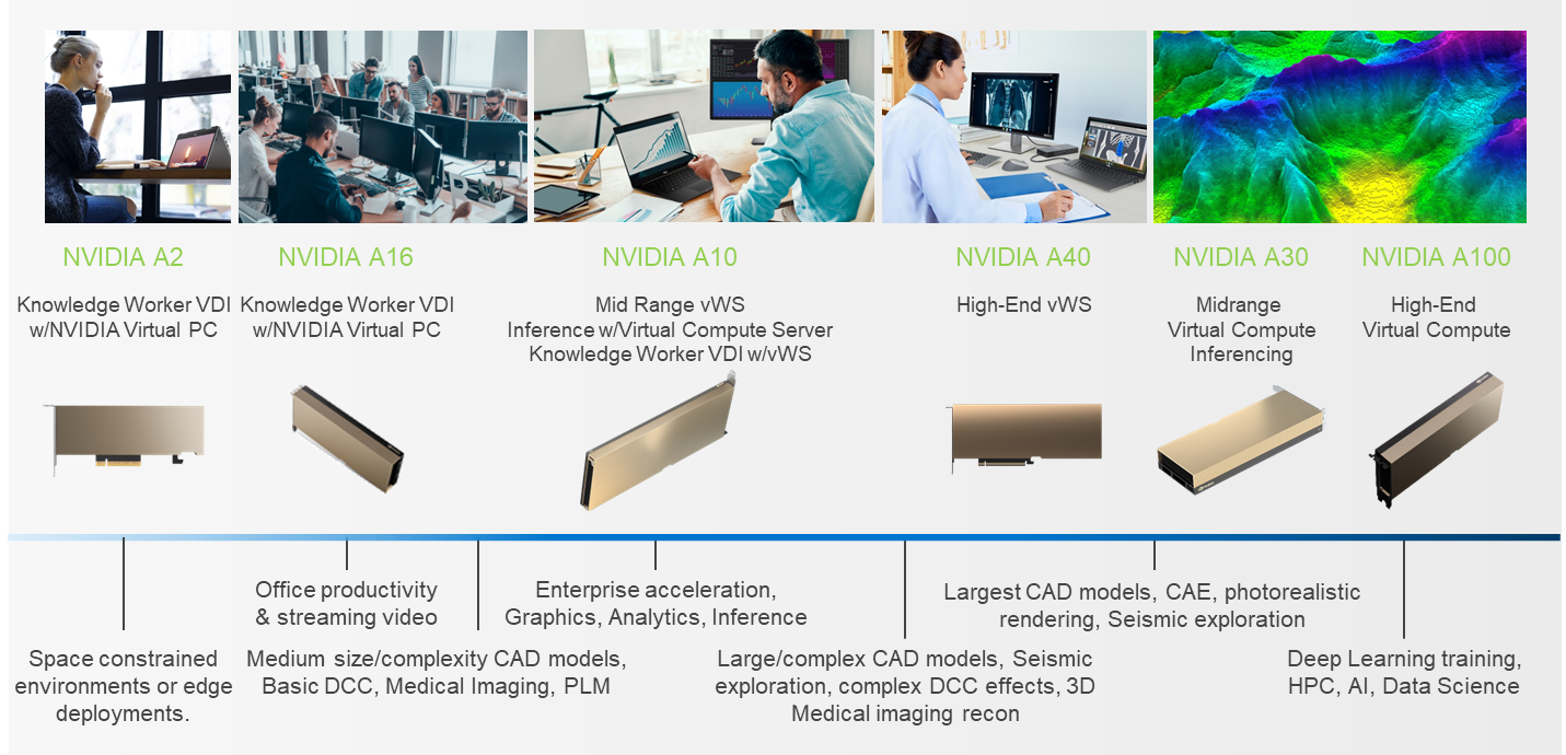
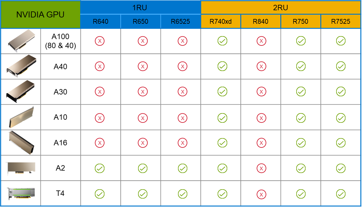
PowerFlex supports a large range of NVIDIA GPUs for workloads, from VDI (Virtual Desktops) to high end virtual compute workloads like AI. You can see this in the following diagram where there are solutions for “space constrained” and “edge” environments, all the way to GPUs used for large inferencing models. In the table below the diagram, you can see which GPUs are supported in each type of PowerFlex node. This provides a tremendous amount of flexibility depending on your workloads.
The validated design describes the steps to configure the architecture and provides detailed links to the NVIDIAand VMware documentation for configuring the vGPUs, and the licensing process for NVIDIA AI Enterprise.
These are key steps when building an AI environment. I know from my experience working with various organizations, and from teaching, that many are not used to working with vGPUs in Linux. This is slowly changing in the industry. If you haven’t spent a lot of time working with vGPUs in Linux, be sure to pay attention to the details provided in the guide. It is important and can make a big difference in your performance.
The following diagram shows the validated design’s logical architecture. At the top of the diagram, you can see four Ubuntu 22.04 Linux VMs with the NVIDIA vGPU driver loaded in them. They are running on PowerFlex hosts with VMware ESXi deployed. Each VM contains one NVIDIA A100 GPU configured for MIG operations. This configuration leverages a two-tier architecture where storage is provided by separate PowerFlex software defined storage (SDS) nodes.
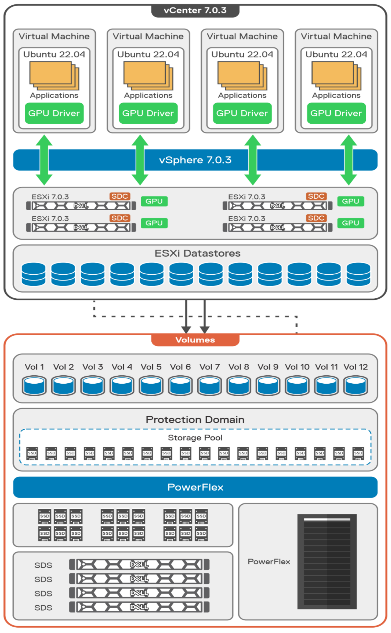
A design like this allows for independent scalability for your workloads. What I mean by this is during the training phase of a model, significant storage may be required for the training data, but once the model clears validation and goes into production, storage requirements may be drastically different. With PowerFlex you have the flexibility to deliver the storage capacity and performance you need at each stage.
This brings us to testing the environment. Again, for this paper, the engineering team validated it using ResNet-50 v1.5 using the ImageNet 1K data set. For this validation they enabled several ResNet-50 v1.5 TensorFlow features. These include Multi-GPU training with Horovod, NVIDIA DALI, and Automatic Mixed Precision (AMP). These help to enable various capabilities in the ResNet-50 v1.5 model that are present in the environment. The paper then describes how to set up and configure ResNet-50 v1.5, the features mentioned above, and details about downloading the ImageNet data.
At this stage they were able to train the ResNet-50 v1.5 deployment. The first iteration of training used the NVIDIA A100-7-40C vGPU profile. They then repeated testing with the A100-4-20C vGPU profile and the A100-3-20C vGPU profile. You might be wondering about the A100-2-10C vGPU profile and the A100-1-5C profile. Although those vGPU profiles are available, they are more suited for inferencing, so they were not tested.
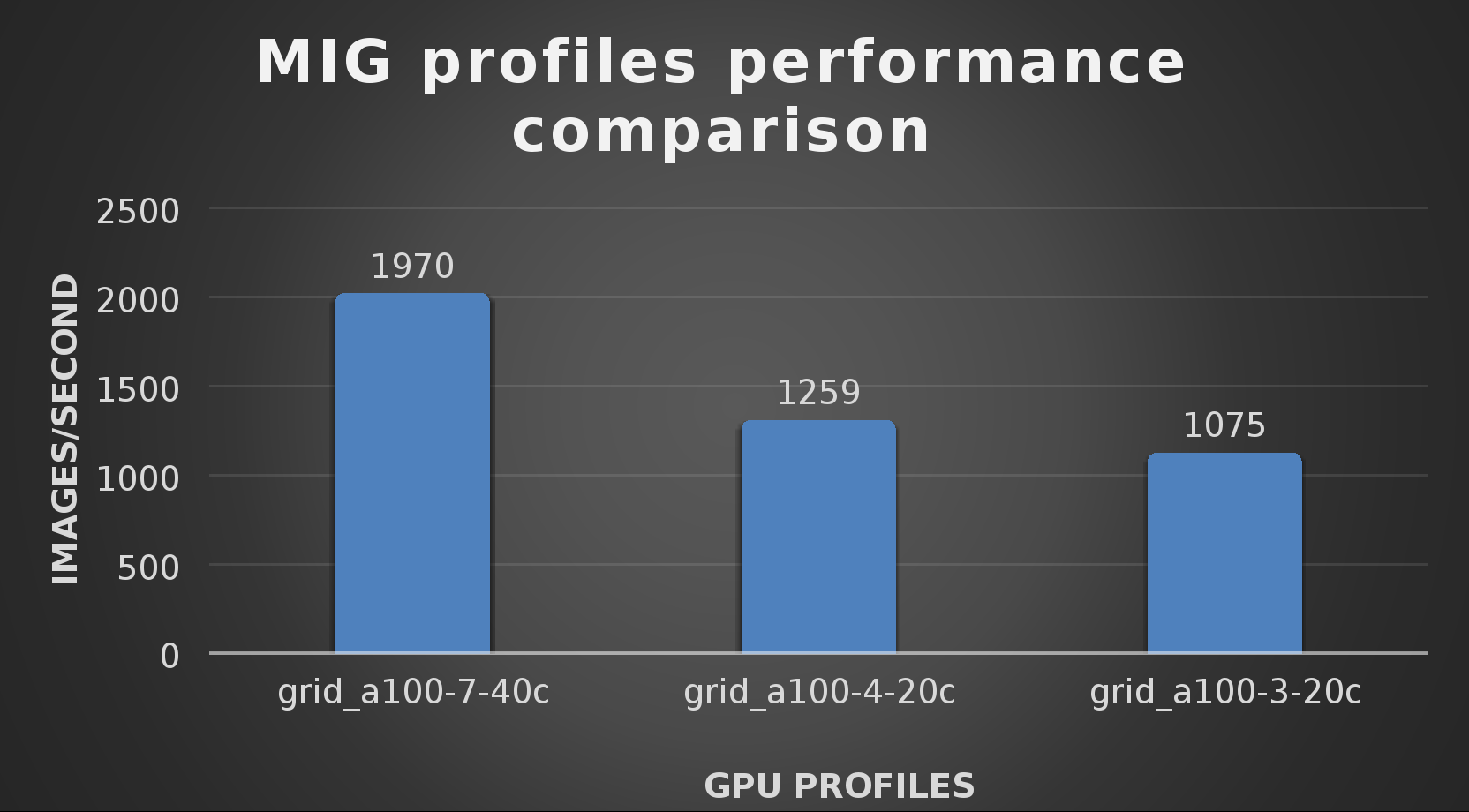
The results from validating the training workloads for each vGPU profile is shown in the following graph. The vGPUs were running near 98% capacity according to nvitop during each test. The CPU utilization was 14% and there was no bottle neck with the storage during the tests.
With the models trained, the guide then looks at how well inference runs on the MIG profiles. The following graph shows inferencing images per second of the various MIG profiles with ResNet-50 v1.5.
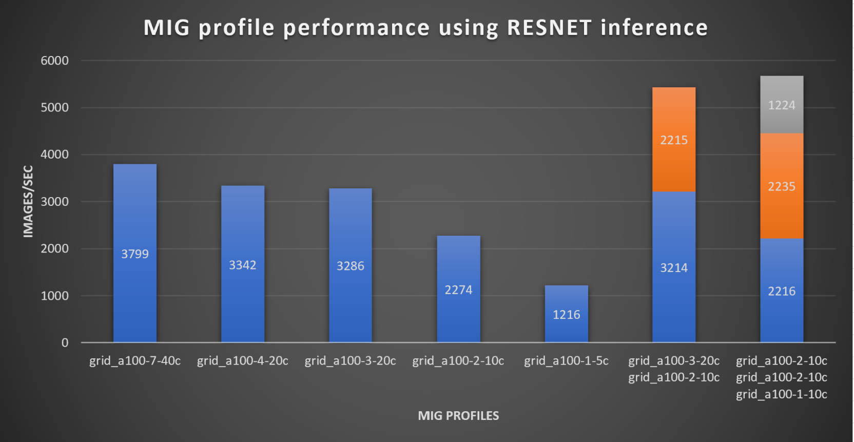
It’s worth noting that the last two columns show the inferencing running across multiple VMs, on the same ESXi host, that are leveraging MIG profiles. This also shows that GPU resources are partitioned with MIG and that resources can be precisely controlled, allowing multiple types of jobs to run on the same GPU without impacting other running jobs.
This opens the opportunity for organizations to align consumption of vGPU resources in virtual environments. Said a different way, it allows IT to provide “show back” of infrastructure usage in the organization. So if a department only needs an inferencing vGPU profile, that’s what they get, no more, no less.
It’s also worth noting that the results from the vGPU utilization were at 88% and CPU utilization was 11% during the inference testing.
These validations show that a Dell PowerFlex environment can support the foundational components of modern-day AI. It also shows the value of NVIDIA’s MIG technology to organizations of all sizes: allowing them to gain operational efficiencies in the data center and enable access to AI.
Which again answers the question of this blog, can I do that AI thing on Dell PowerFlex… Yes you can run that AI thing! If you would like to find out more about how to run your AI thing on PowerFlex, be sure to reach out to your Dell representative.
Resources
- The History of Artificial Intelligence
- ‘Godfather of AI’ leaves Google, warns of tech’s dangers
- ResNet-50: The Basics and a Quick Tutorial
- Dell Validated Design for Virtual GPU with VMware and NVIDIA on PowerFlex
- NVIDIA NGC Catalog ResNet v1.5 for PyTorch
- NVIDIA AI Enterprise
- NVIDIA A100 (PCIe) GPU
- NVIDIA Virtual GPU Software Documentation
- NVIDIA A100-7-40C vGPU profile
- NVIDIA Multi-Instance GPU (MIG)
- NVIDIA Multi-Instance GPU User Guide
- Horovod
- ImageNet
- DALI
- Automatic Mixed Precision (AMP)
- nvitop
Author: Tony Foster
Sr. Principal Technical Marketing Engineer
Twitter: | |
LinkedIn: | |
Personal Blog: | |
Location: | The Land of Oz [-6 GMT] |