


LAMMPS — with Ice Lake on Dell EMC PowerEdge Servers
3rd Generation Intel Xeon® Scalable processors (architecture code named Ice Lake) is Intel’s successor to Cascade Lake. New features include up to 40 cores per processor, eight memory channels with support for 3200 MT/s memory speed and PCIe Gen4. The HPC and AI Innovation Lab at Dell EMC had access to a few systems and this blog presents the results of our initial benchmarking study.
LAMMPS Overview
Large-scale Atomic/Molecular Massively Parallel Simulator (LAMMPS) is an open source, well parallelized collection of packages for molecular dynamics (MD) research. LAMMPS has a nice collection of “atom styles”, force fields, and many contributed packages. LAMMPS can run on a single processor or on the largest parallel super-computers. It also has packages that provide force calculations accelerated on GPU’s. It can do simulations with billions of atoms!
LAMMPS can be run on a single processor or in parallel using some form of message passing, such as Message Passing Interface (MPI). The most current source code for LAMMPS is written in C++. For more information about LAMMPS, see the following link: https://www.lammps.org/.
Objective
In this study we measure the performance of LAMMPS on different Ice Lake processor models as listed in Table 1 with a comparison to the previous generation Cascade Lake systems. Single node as well as the multi-node scalability tests were conducted.
Compilation Details
The LAMMPS version used for testing release was lammps-2July-2021, using the Intel 2020 update 5 compiler to take advantage of AVX2 and AVX512 optimizations, and the Intel MKL FFT library. We used the default INTEL package, which comes along the LAMMPS package providing some well optimized atom pair styles in LAMMPS for the vector instructions on Intel processors. The datasets used for our study are described in Table 2, along with detailed configuration of atom sizes and run steps. The unit of performance is timesteps per second, and higher is better.
Hardware and software configurations
Table 1: Hardware and Software test bed details
Component | Dell EMC PowerEdge R750 server | Dell EMC PowerEdge R750 server | Dell EMC PowerEdge C6520 server | Dell EMC PowerEdge C6520 server | Dell EMC PowerEdge C6420 server | Dell EMC PowerEdge C6420 server |
CPU model | Xeon 8380 | Xeon 8358 | Xeon 8352Y | Xeon 6330 | Xeon 8280 | Xeon 6248R |
Cores/Socket | 40 | 32 | 32 | 28 | 28 | 24 |
Base Frequency | 2.30 GHz | 2.60 GHz | 2.20 GHz | 2.00 GHz | 2.70 GHz | 3.00 GHz |
TDP | 270 W | 250 W | 205 W | 205 W | 205 W | 205 W |
Operating System | Red Hat Enterprise Linux 8.3 4.18.0-240.22.1.el8_3.x86_64 | |||||
Memory |
16 GB x 16 (2Rx8) 3200 MT/s
| 16 GB x 12 (2Rx8) 2933 MT/s | ||||
BIOS/CPLD | 1.1.2/1.0.1 | |||||
Interconnect | NVIDIA Mellanox HDR
| NVIDIA Mellanox HDR100 | ||||
Compiler | Intel parallel studio 2020 (update 4) | |||||
LAMMPS | 2july2021 | |||||
Datasets used for performance analysis
Table 2: Description of datasets used for performance analysis
Datasets | Description | Units | Atomic Style | Atom Size | Step Size |
Lennard Jones | Atomic fluid (LJ Benchmark) | lj | atomic | 512000 | 7900 |
Rhodo | Protein (Rhodopsin Benchmark) | real | full | 512000 | 520 |
Liquid crystal | Liquid Crystal w/ Gay-Berne potential | lj | ellipsoid | 524288 | 840 |
Eam | Copper benchmark with Embedded Atom Method | metal | atomic | 512000 | 3100 |
Stilliger Weber | Silicon benchmark with Stillinger-Weber | metal | atomic | 512000 | 6200 |
Tersoff | Silicon benchmark with Tersoff | metal | atomic | 512000 | 2420 |
Water | Coarse-grain water benchmark using Stillinger-Weber | real | atomic | 512000 | 2600 |
Polyethylene | Polyethylene benchmark with AIREBO | metal | atomic | 522240 | 550 |
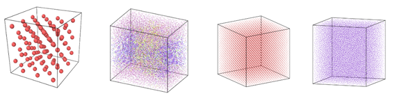
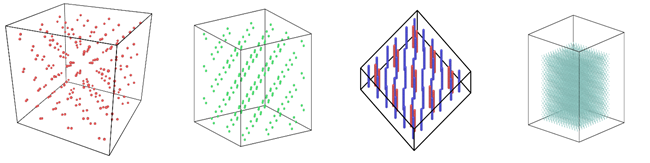
Figure 1: Image view of datasets from OVITO (scientific data visualization and analysis software for molecular and other particle-based simulation model). Images are listed in order 1a-1h, subfigure 1a- 1h represents a small portion of simulation domain for Atomic Fluid (Lennard Jones), rhodo(protein), liquid crystal(lc), copper(eam), stilliger webner(sw), Terasoff, water, polyethylene datasets respectively.
Table 1 and Figure 1 shows the image view of datasets used for the single and multi-node analysis. For visualization of all datasets was done using OVITO, scientific data visualization and analysis software for molecular and other particle-based simulation model. For single node performance study, all the datasets shown in Table 2 were used, and for multi-node study Atomic fluid was considered for benchmarking.
Performance Analyses on Single Node
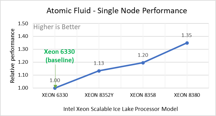
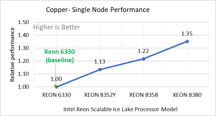
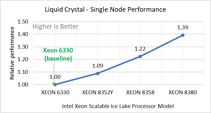
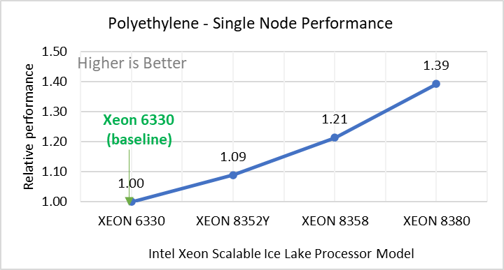
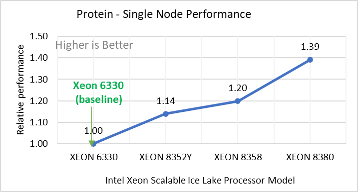
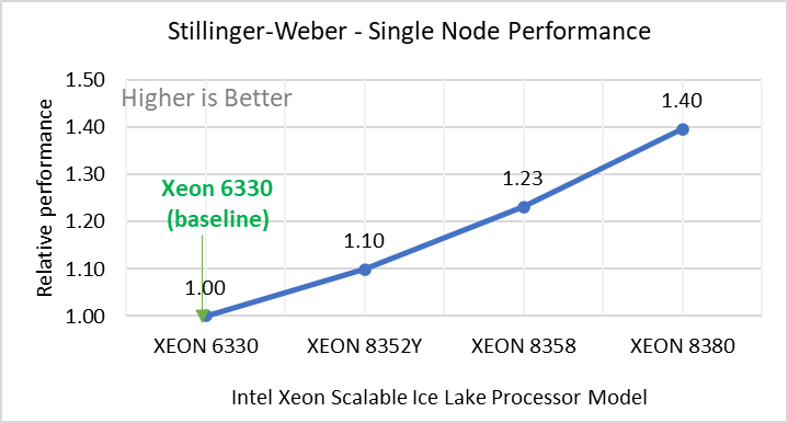
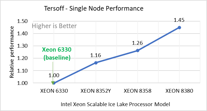
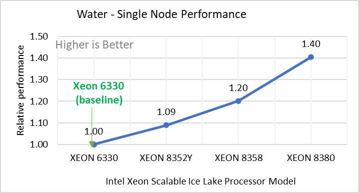
Figure 2: Single Node Performance of LAMMPS across the datasets with Intel Ice Lake processor model. Each graph in Figure 2 is an individual subfigure, labeled (a-h) in the order shown. Each subfigure (2a- 2h) represents single node performance comparison across the Xeon processors with Xeon 6330 as baseline for Atomic Fluid (Lennard Jones), rhodo(protein), liquid crystal(lc), copper(eam), stilliger webner(sw), Terasoff, water, polyethylene datasets respectively.
Figure 2 shows the single node performance for the eight datasets (sub figure 2a-h) listed in Table 2 with the four Ice Lake processor model available for evaluation of LAMMPS.
For ease of comparison across the processor model, the relative performance of the datasets has been included into a different graph. However, it is worth noting that each dataset behaves individually when performance is considered, as each uses different molecular potentials and have different number of atoms. Figure 2 shows that increases in the core count in the processor model increases the performance, across the dataset used. Next, by comparing the relative numbers to the baseline processor Xeon 6330(28C) with Xeon 8380(40C), we measured a 30 to 45 percent performance gain with these datasets. A fraction of these boosts was due to frequency of the processor model.
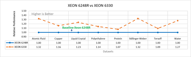
Figure 3a: Performance of LAMMPS on Cascade Lake (Xeon 6248R) in comparison to Ice Lake (Xeon 6330)
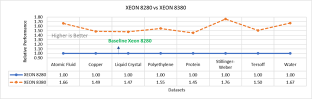
Figure 3b: Performance of LAMMPS on Cascade Lake (Xeon 8280) in comparison to Ice Lake (Xeon 8380)
Figure 3 compares the performance of the mid-bin Cascade Lake 6248R (24core) to the Ice Lake 6330 (28 core), and the top end Cascade Lake 8280 (28 core) to the Ice Lake 8380 (40 core) From the figure 3a, Ice Lake 6330 is up to 30 percent faster than the 6248R. The Xeon 6330 has 16 percent more cores, and 9 percent faster memory bandwidth. Figure 3b shows Ice Lake 8380 is up to 75 percent faster than the Xeon 8280 on single node tests, this is in line with the 42 percent additional cores and 9 percent faster memory bandwidth. These results are due to a higher processor speed wherein more data can be accessed by each core.
Performance Analysis on Multi-Node
To analyze the scalability test with strong and weak scaling, we used the Atom Fluid (LJ) dataset from the Intel package. The job run time was 7900 steps with 512000 atoms in the simulation system.
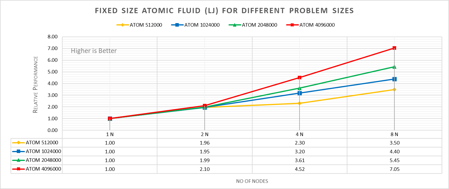
Figure 4a: Fixed size Atomic fluid (LJ) for different problem size (strong scaling) w/ Xeon 8380
With strong scaling, we referred to the fixed problem size and increasing the parallel processes (Amdahl’s law). Whereas in weak scaling, we varied the atom size from 512000 atoms to 4096000 atoms in the simulation environment with an increase in the parallel processes (Gustafson-Barsis law). The test bed included DellEMC Poweredge R750 servers each with dual Ice Lake Xeon 8380 processors an NVIDIA Networking HDR interconnect running at 200 Gbps.Figure 4a plots the fixed-size relative performance for four different problem sizes, viz, 512000,1024000,2048000, and 4096000 atoms, on different number of nodes.
The relative performance is normalized by single node performance. Hence, the single node performance for each curve is 1.00 (unity). Relative Performance for fixed size Atomic fluid was calculated by the following equation:
Relative Performance = loop time of ‘N’ node / loop time for single node
Loop time is the total wall-clock time for the simulation to run. It can be observed that relative performance increases with increase in problem size. This is because for smaller problems system spend more time in inter-nodal communications. Time spent in communication at 8 nodes is 61.91%, 59.74%,48.42%,45.04% for 512000,1024000,2048000,4096000 atom size respectively.
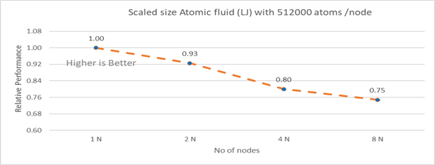
Figure 4b: Scaled size Atomic fluid (LJ) with 512000 atoms per node (weak scaling) w/ Xeon 8380
Figure 4b plots the scaled-size efficiency for runs with 512000 atoms per node. Thus, a scaled-size 2 node run is for 1024000 atoms; 8 node runs is for 4096000 atoms. Relative Performance for Scaled size Atomic fluid was calculated by the following equation:
Relative Performance= loop time for ‘n’ node/ (loop time for single node * number of nodes)
Weak scaling efficiency decreases with increase in no of nodes in the investigated range. This is due to the fact for larger number of nodes the time spend in MPI communication is larger. Time spent in communication with scaled size atom for 1N, 2N, 4N and 8 N are 27.17%, 32.42 %, 40.87%, 45.04 % respectively.
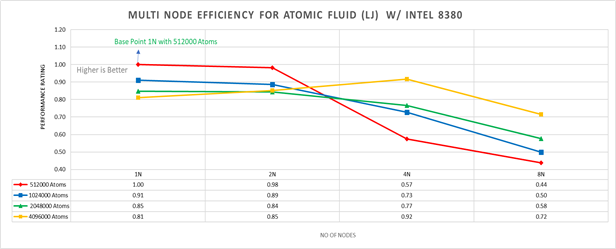
Figure 5: Multi-node efficiency for Atomic Fluid (LJ) w/ I 8380
Figure 5 plots the multi-node efficiency for Atomic Fluid with Xeon 8380. The relative performance is normalized by single node with 512000 atoms performance. Hence, the single node performance for 512000 atoms is 1.00 (unity). This point is taken as baseline for other comparison.
Performance Rating = (loop time * number of atoms)/ (loop time for 512000 atoms on 1 node * number of nodes * 512000)
We observed that for smaller systems, such as those with fewer atoms, the efficiency of strong scaling decreases as the system spends more time in MPI communication; whereas in larger systems with many atoms, the efficiency of strong scaling increases as the time spent in pair-wise force calculation becomes dominant. For weak scaling, as the no of nodes increases the efficiency of weak scaling decreases.
Conclusion
The Ice Lake processor-based Dell EMC Power Edge servers, with its hardware feature upgrades over Cascade Lake, demonstrate up to 50 to70 percent performance gain for all the datasets used for benchmarking LAMMPS. Watch our blog site for updates!
Related Blog Posts

MD Simulation of GROMACS with AMD EPYC 7003 Series Processors on Dell EMC PowerEdge Servers
Thu, 19 Aug 2021 20:06:53 -0000
|Read Time: 0 minutes
AMD has recently announced and launched its third generation 7003 series EPYC processors family (code named Milan). These processors build upon the proceeding generation 7002 series (Rome) processors and improve L3 cache architecture along with an increased memory bandwidth for workloads such as High Performance Computing (HPC).
The Dell EMC HPC and AI Innovation Lab has been evaluating these new processors with Dell EMC’s latest 15G PowerEdge servers and will report our initial findings for the molecular dynamics (MD) application GROMACs in this blog.
Given the enormous health impact of the ongoing COVID-19 pandemic, researchers and scientists are working closely with the HPC and AI Innovation Lab to obtain the appropriate computing resources to improve the performance of molecular dynamics simulations. Of these resources, GROMACS is an extensively used application for MD simulations. It has been evaluated with the standard datasets by combining the latest AMD EPYC Milan processor (based on Zen 3 cores) with Dell EMC PowerEdge servers to get most out of the MD simulations.
In a previous blog, Molecular Dynamic Simulation with GROMACS on AMD EPYC- ROME, we published benchmark data for a GROMACS application study on a single node and multinode with AMD EPYC ROME based Dell EMC servers.
The results featured in this blog come from the test bed described in the following table. We performed a single-node and multi-node application study on Milan processors, using the latest AMD stack shown in Table 1, with GROMACS 2020.4 to understand the performance improvement over the older generation processor (Rome).
Table 1: Testbed hardware and software details
Server | Dell EMC PowerEdge 2-socket servers (with AMD Milan processors) | Dell EMC PowerEdge 2-socket servers (with AMD Rome processors) |
Processor Cores/socket Frequency (Base-Boost ) Default TDP Processor bus speed | 7763 (Milan) 64 2.45 GHz – 3.5 GHz 280 W 256 MB 16 GT/s | 7H12 (Rome) 64 2.6 GHz – 3.3 GHz 280 W 256 MB 16 GT/s |
Processor Cores/socket Frequency Default TDP Processor bus speed | 7713 (Milan) 64 2.0 GHz – 3.675 GHz 225 W 256 MB 16 GT/s | 7702 (Rome) 64 2.0 GHz – 3.35 GHz 200 W 256 MB 16 GT/s |
Processor Cores/socket Frequency Default TDP Processor bus speed | 7543 (Milan) 32 2.8 GHz – 3.7 GHz 225 W 256 MB 16 GT/s | 7542 (Rome) 32 2.9 GHz – 3.4 GHz 225 W 128 MB 16 GT/s |
Operating system | Red Hat Enterprise Linux 8.3 (4.18.0-240.el8.x86_64) | Red Hat Enterprise Linux 7.8 |
Memory | DDR4 256 G (16 GB x 16) 3200 MT/s | |
BIOS/CPLD | 2.0.2 / 1.1.12 |
|
Interconnect | NVIDIA Mellanox HDR | NVIDIA Mellanox HDR 100 |
Table 2: Benchmark datasets used for GROMACS performance evaluation
Datasets | Details |
1536 K and 3072 K | |
1400 K and 3000 K | |
Prace – Lignocellulose | 3M |
The following information describes the performance evaluation for the processor stack listed in the Table 1.
Rome processors compared to Milan processors (GROMACS)
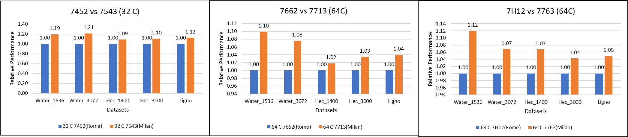 Figure 1: GROMACS performance comparison with AMD Rome processors
For performance benchmark comparisons, we selected Rome processors that are closest to their Milan counterparts in terms of hardware features such as cache size, TDP values, and Processor Base/Turbo Frequency, and marked the maximum value attained for Ns/day by each of the datasets mentioned in Table 2.
Figure 1 shows a 32C Milan processor has higher performance improvements (19 percent for water 1536, 21 percent for water 3072, and 10 to approximately 12 percent with HECBIO sim and lingo cellulose datasets) compared to a 32C Rome processor. This result is due to a higher processor speed and improved L3 cache, wherein more data can be accessed by each core.
Next, with the higher end processor we see only 10 percent gain with respect to the water dataset, as they are more memory intensive. Some percentage is added on due to improvement of frequency for the remaining datasets. Overall, the Milan processor results demonstrated a substantial performance improvement for GROMACS over Rome processors.
Milan processors comparison (32C processors compared to 64C processors)
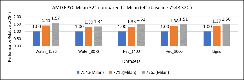
Figure 2: GROMACS performance with Milan processors
Figure 2 shows performance relative to the performance obtained on the 7543 processor. For instance, the performance of water 1536 is improved from the 32C processor to the 64 core (64C) processor from 41 percent (7713 processor) to 57 percent (7763 processor). The performance improvement is due to the increasing core counts and higher CPU core frequency performance improvement. We observed that GROMACS is frequency sensitive, but not to a great extent. Greater gains may be seen when running GROMACS across multiple ensembles runs or running dataset with higher number of atoms.
We recommend that you compare the price-to-performance ratio before choosing the processor based on the datasets with higher CPU core frequency, as the processors with a higher number of lower-frequency cores may provide better total performance.
Multi-node study with 7713 64C processors
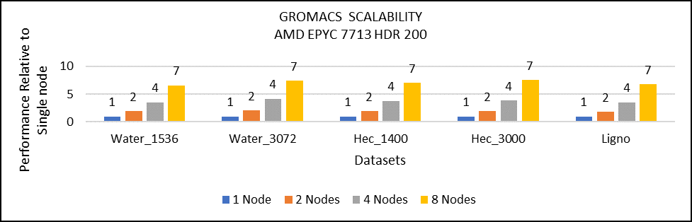
Figure 3: Multi-node study with 7713 64c SKUs
For multi-node tests, the test bed was configured with an NVIDIA Mellanox HDR interconnect running at 200 Gbps and each server included an AMD EPYC 7713 processor. We achieved the expected linear performance scalability for GROMACS of up to four nodes and across each of the datasets. All cores in each server were used while running the benchmarks. The performance increases are close to linear across all the dataset types as core count increases.
Conclusion
For the various datasets we evaluated, GROMACS exhibited strong scaling and was compute intensive. We recommend a processor with high core count for smaller datasets (water 1536, hec 1400); larger datasets (water 3072, ligno,HEC 3000) would benefit from memory per core. Configuring the best BIOS options is important to get the best performance out of the system.
For more information and updates, follow this blog site.

Intel Ice Lake - BIOS Characterization for HPC
Tue, 25 May 2021 13:10:03 -0000
|Read Time: 0 minutes
Intel recently announced the 3rd Generation Intel Xeon Scalable processors (code-named “Ice Lake”), which are based on a new 10 nm manufacturing process. This blog provides the new Ice Lake processor synthetic benchmark results and the recommended BIOS settings on Dell EMC PowerEdge servers.
Ice Lake processors offer a higher core count of up to 40 cores with a single Ice Lake 8380 processor. The Ice Lake processors have larger L3, L2, and L1 data cache than Intel’s second-generation Cascade Lake processors. These features are expected to improve performance of CPU-bound software applications. Table 1 shows the L1, L2, and L3 cache size on the 8380 processor model.
Ice Lake still supports the AVX 512 SIMD instructions, which allow for 32 DP FLOP/cycle. The upgraded Ultra Path Interconnect (UPI) Link speed of 11.2GT/s is expected to improve data movement between the sockets. In addition to core count and frequency, Ice Lake-based Dell EMC PowerEdge servers support DDR4 - 3200 MT/s DIMMS with eight memory channels per processor, which is expected to improve the performance of memory bandwidth-bound applications. Ice Lake processors now support DIMMs with 6 TB per socket.
Instructions such as Vector CLMUL, VPMADD52, Vector AES, and GFNI Extensions have been optimized to improve use of vector registers. The performance of software applications in the cryptography domain is also expected to benefit. The Ice Lake processor also includes improvements to Intel Speed Select Technology (Intel SST). With Intel SST, a few cores from the total available cores can be operated at a higher base frequency, turbo frequency, or power. This blog does not address this feature.
Table 1: hwloc-ls and numactl -H command output on an Intel 8380 processor model-based server with Round Robin core enumeration (MadtCoreEnumeration) and SubNumaCuster(Sub-NUMA Cluster) set to 2-Way
hwloc-ls | numactl -H |
Machine (247GB total) Package L#0 + L3 L#0 (60MB) Group0 L#0 NUMANode L#0 (P#0 61GB) L2 L#0 (1280KB) + L1d L#0 (48KB) + L1i L#0 (32KB) + Core L#0 + PU L#0 (P#0) L2 L#1 (1280KB) + L1d L#1 (48KB) + L1i L#1 (32KB) + Core L#1 + PU L#1 (P#4) L2 L#2 (1280KB) + L1d L#2 (48KB) + L1i L#2 (32KB) + Core L#2 + PU L#2 (P#8) L2 L#3 (1280KB) + L1d L#3 (48KB) + L1i L#3 (32KB) + Core L#3 + PU L#3 (P#12) L2 L#4 (1280KB) + L1d L#4 (48KB) + L1i L#4 (32KB) + Core L#4 + PU L#4 (P#16) L2 L#5 (1280KB) + L1d L#5 (48KB) + L1i L#5 (32KB) + Core L#5 + PU L#5 (P#20) L2 L#6 (1280KB) + L1d L#6 (48KB) + L1i L#6 (32KB) + Core L#6 + PU L#6 (P#24) L2 L#7 (1280KB) + L1d L#7 (48KB) + L1i L#7 (32KB) + Core L#7 + PU L#7 (P#28) L2 L#8 (1280KB) + L1d L#8 (48KB) + L1i L#8 (32KB) + Core L#8 + PU L#8 (P#32) L2 L#9 (1280KB) + L1d L#9 (48KB) + L1i L#9 (32KB) + Core L#9 + PU L#9 (P#36) L2 L#10 (1280KB) + L1d L#10 (48KB) + L1i L#10 (32KB) + Core L#10 + PU L#10 (P#40) L2 L#11 (1280KB) + L1d L#11 (48KB) + L1i L#11 (32KB) + Core L#11 + PU L#11 (P#44) L2 L#12 (1280KB) + L1d L#12 (48KB) + L1i L#12 (32KB) + Core L#12 + PU L#12 (P#48) L2 L#13 (1280KB) + L1d L#13 (48KB) + L1i L#13 (32KB) + Core L#13 + PU L#13 (P#52) L2 L#14 (1280KB) + L1d L#14 (48KB) + L1i L#14 (32KB) + Core L#14 + PU L#14 (P#56) L2 L#15 (1280KB) + L1d L#15 (48KB) + L1i L#15 (32KB) + Core L#15 + PU L#15 (P#60) L2 L#16 (1280KB) + L1d L#16 (48KB) + L1i L#16 (32KB) + Core L#16 + PU L#16 (P#64) L2 L#17 (1280KB) + L1d L#17 (48KB) + L1i L#17 (32KB) + Core L#17 + PU L#17 (P#68) L2 L#18 (1280KB) + L1d L#18 (48KB) + L1i L#18 (32KB) + Core L#18 + PU L#18 (P#72) L2 L#19 (1280KB) + L1d L#19 (48KB) + L1i L#19 (32KB) + Core L#19 + PU L#19 (P#76) HostBridge. <snip> . .
| |
BIOS options tested on Ice Lake processors
Table 2 provides the server details used for the performance tests. The following BIOS options were explored in the performance testing:
- BIOS.ProcSettings.SubNumaCluster—Breaks up the LLC into disjoint clusters based on address range, with each cluster bound to a subset of the memory controllers in the system. It improves average latency to the LLC. Sub-NUMA Cluster (SNC) is disabled if NVDIMM-N is installed in the system.
- BIOS.ProcSettings.DeadLineLlcAlloc—If enabled, fills in dead lines in LLC opportunistically.
- BIOS.ProcSettings.LlcPrefetch—Enables and disables LLC Prefetch on all threads.
- BIOS.ProcSettings.XptPrefetch—If enabled, enables the MS2IDI to take a read request that is being sent to the LLC and speculatively issue a copy of that read request to the memory controller.
- BIOS.ProcSettings.UpiPrefetch—Starts the memory read early on the DDR bus. The UPI Rx path spawns a MemSpecRd to iMC directly.
- BIOS.ProcSettings.DcuIpPrefetcher (Data Cache Unit IP Prefetcher)—Affects performance, depending on the application running on the server. This setting is recommended for High Performance Computing applications.
- BIOS.ProcSettings.DcuStreamerPrefetcher (Data Cache Unit Streamer Prefetcher)—Affects performance, depending on the application running on the server. This setting is recommended for High Performance Computing applications.
- BIOS.ProcSettings.ProcAdjCacheLine—When set to Enabled, optimizes the system for applications that require high utilization of sequential memory access. Disable this option for applications that require high utilization of random memory access.
- BIOS.SysProfileSettings.SysProfile—Sets the System Profile to Performance Per Watt (DAPC), Performance Per Watt (OS), Performance, Workstation Performance, or Custom mode. When set to a mode other than Custom, the BIOS sets each option accordingly. When set to Custom, you can change setting of each option.
- BIOS.ProcSettings.LogicalProc—Reports the logical processors. Each processor core supports up to two logical processors. When set to Enabled, the BIOS reports all logical processors. When set to Disabled, the BIOS only reports one logical processor per core. Generally, a higher processor count results in increased performance for most multithreaded workloads. The recommendation is to keep this option enabled. However, there are some floating point and scientific workloads, including HPC workloads, where disabling this feature might result in higher performance.
You can set the DeadLineLlcAlloc, LlcPrefetch, XptPrefetch, UpiPrefetch, DcuIpPrefetcher, DcuStreamerPrefetcher, ProcAdjCacheLine, and LogicalProc BIOS options to either Enabled or Disabled. You can set the SubNumaCluster to 2-Way and Disabled. The SysProfile setting can have five possible values: PerformanceOptimized, PerfPerWattOptimizedDapc, PerfPerWattOptimizedOs, PerfWorkStationOptimized and Custom.
Table 2: Test bed hardware and software details
Component | Dell EMC PowerEdge R750 server | Dell EMC PowerEdge C6520 server | Dell EMC PowerEdge C6420 server | Dell EMC PowerEdge C6420 server |
OPN | 8380 | 6338 | 8280 | 6252 |
Cores/Socket | 40 | 32 | 28 | 24 |
Frequency (Base-Boost) | 2.30 – 3.40 GHz | 2.0 – 3.20 GHz | 2.70 – 4.0 GHz | 2.10 – 3.70 GHz |
TDP | 270 W | 205 W | 205 W | 150 W |
L3Cache | 60M | 48M | 38.5M | 37.75M |
Operating System | Red Hat Enterprise Linux 8.3 4.18.0-240.22.1.el8_3.x86_64 | Red Hat Enterprise Linux 8.3 4.18.0-240.22.1.el8_3.x86_64 | Red Hat Enterprise Linux 8.3 4.18.0-240.el8.x86_64 | Red Hat Enterprise Linux 8.3 4.18.0-240.el8.x86_64 |
Memory | 16 GB x 16 (2Rx8) 3200 MT/s | 16 GB x 16 (2Rx8) 3200 MT/s | 16 GB x 12 (2Rx8) 2933 MT/s | 16 GB x 12 (2Rx8) 2933 MT/s |
BIOS/CPLD | 1.1.2/1.0.1 | |||
Interconnect | NVIDIA Mellanox HDR | NVIDIA Mellanox HDR | NVIDIA Mellanox HDR100 | NVIDIA Mellanox HDR100 |
Compiler | Intel parallel studio 2020 (update 4) | |||
Benchmark software |
| |||
The system profile BIOS meta option helps to set a group of BIOS options (such as C1E, C States, and so on), each of which control performance and power management settings to a particular value. It is also possible to set these groups of BIOS options individually to a different value using the Custom system profile.
Application performance results
Table 2 lists details about the software used for benchmarking the server. We used the precompiled HPL and HPCG binary files, which are part of Intel Parallel Studio 2020 update 4 software bundle, for our tests. We compiled the WRF application with AVX2 support. WRF and HPCG issue many nonfloating point packed micro-operations (approximately 73 percent to 90 percent of the total packed micro-operations). They are memory-bound (and DRAM-bandwidth bound) workloads. HPL issues packed double precision micro-operations and is a compute-bound workload.
After setting Sub-NUMA Cluster (BIOS.ProcSettings.SubNumaCluster) to 2-Way, Logical Processors (BIOS.ProcSettings.LogicalProc) to Disabled, and other settings (DeadLineLlcAlloc, LlcPrefetch, XptPrefetch, UpiPrefetch, DcuIpPrefetcher, DcuStreamerPrefetcher, ProcAdjCacheLine) to Enabled, we measured the impact of System Profile (BIOS.SysProfileSettings.SysProfile) BIOS parameters on application performance.
Figure 1 through Figure 4 show application performance. In each figure, the numbers over the bars represent the relative change in the application performance with respect to the application performance obtained on the Intel 6338 Ice Lake processor with the System Profile set to Performance Optimized (PO).
Note: In the figures, PO=PerformanceOptimized, PPWOD=PerfPerWattOptimizedDapc, PPWOO=PerfPerWattOptimizedOs, and PWSO=PerfWorkStationOptimized.
HPL Benchmark
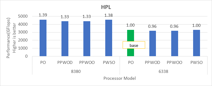
Figure 1: Relative difference in the performance of HPL by processor and Sysprofile setting
HPCG Benchmark
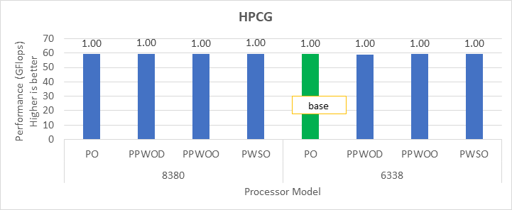
Figure 2: Relative difference in the performance of HPCG by processor and Sysprofile setting
STREAM Benchmark
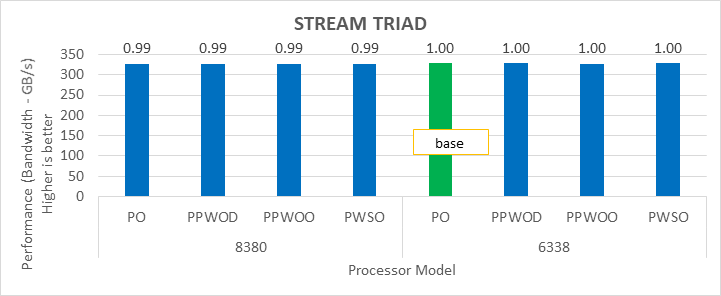
Figure 3: Relative difference in the performance of STREAM by processor and Sysprofile setting
WRF Benchmark
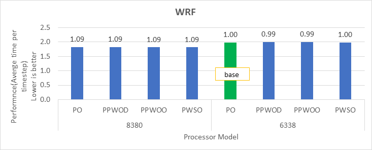
Figure 4: Relative difference in the performance of WRF by processor and Sysprofile setting
We obtained the performance for the applications in Figure 2 through Figure 4 by fully subscribing to all available cores. Depending on the processor model, we achieved 78 percent to 80 percent efficiency with HPL and STREAM benchmarks using the Performance Optimized profile.
Intel has extended the TDP of the Ice Lake processors with the top-end Intel 8380 processor at 270 W TDP. The following figure shows the power use on the systems with the applications listed in Table 2.Note: In this figure, PO=PerformanceOptimized, PPWOD=PerfPerWattOptimizedDapc, PPWOO=PerfPerWattOptimizedOs and PWSO=PerfWorkStationOptimized
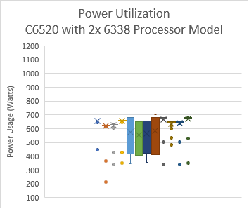
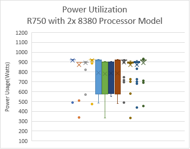
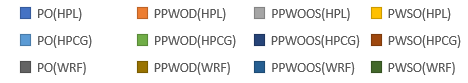
Figure 5: Power use by platform and processor type. Average Idle power usage on the PowerEdge C6520 server (Intel 6338 processor) with approximately 335 W and the PowerEdge R750 server (intel 8380 processor) with approximately 470 W using the Performance Optimized System Profile.
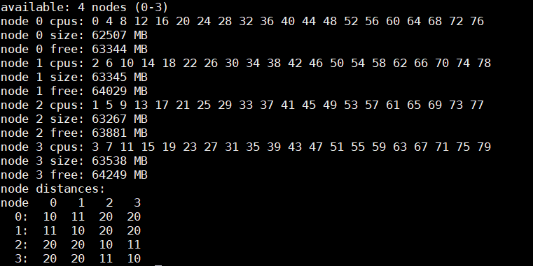
When SNC is set to 2-Way, the system exposes four NUMA nodes. We tested the NUMA bandwidth, remote socket bandwidth, and local socket bandwidth using the STREAM TRIAD benchmark. In Figure 6, the CPU NUMA node is represented as c and the memory node is represented as m. As an example for NUMA bandwidth, the c0m0 (blue bars) test type represents the STREAM TRIAD test carried out between NUMA node 0 and memory node 0. Figure 6 shows the best bandwidth numbers obtained on varying the number of threads per test type.
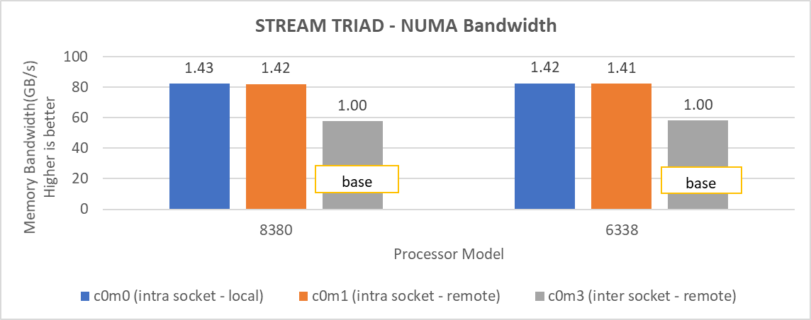
Figure 6: Local and remote NUMA memory bandwidth.
Remote socket bandwidth numbers were measured between CPU node 0, 1 and memory node 2, 3. Local bandwidths were measured between CPU node 0, 1, and 0, 1. The following figure shows the performance numbers.
Figure 7: Local and remote processor bandwidth.
Impact of BIOS options on application performance
We tested the impact of the DeadLineLlcAlloc, LlcPrefetch, XptPrefetch, UpiPrefetch, DcuIpPrefetcher, DcuStreamerPrefetcher and ProcAdjCacheLine with the Performance Optimized (PO) system profile. These BIOS options do not have significant impact on the performance of applications addressed in this blog, therefore we recommend that these options be set as Enabled.
Figure 8 and Figure 9 show the impact of the Sub-NUMA Cluster (SNC) BIOS option on the application performance. In each figure, the numbers over the bars represent the relative change in the application performance with respect to the application performance obtained on the Intel 6338 Ice Lake processor with SNC feature set to Disabled.
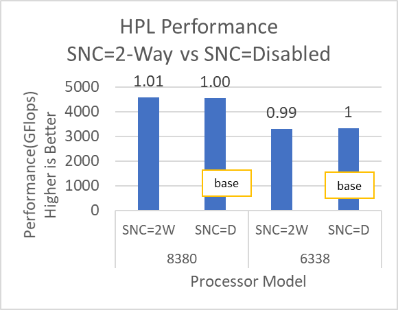
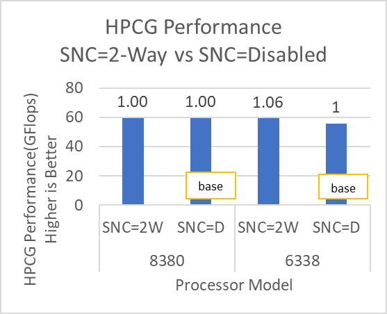
Figure 8: HPL and HPCG performance variation by processor model with Sub-NUMA Cluster set to Disabled (SNC=D) and 2-Way (SNC=2W)
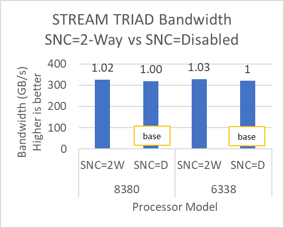
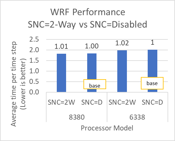
Figure 9: STREAM and WRF performance variation by processor model with Sub-NUMA Cluster set to Disabled (SNC=D) and 2-Way (SNC=2W)
The SubNumaCluster option can impact the applications that are Memory Bandwidth-bound (for example, STREAM, HPCG, and WRF). The SubNumaCluster option is recommended to be set to 2-Way as it can optimize the workloads addressed in this blog by a range of one percent to six percent, depending on the processor model and application.
InfiniBand bandwidth and message rate
The Ice Lake-based processors now support PCIe Gen 4, which allows the NVIDIA MELLANOX HDR adapter cards to be used with Dell EMC PowerEdge servers. Figure 10, Figure 11, and Figure 12 show the Message Rate, Unidirectional, and Bi-directional InfiniBand bandwidth test results of the OSU Benchmarks suite. The network adapter card was connected to the second socket (NUMA node 2), therefore, the local bandwidth tests were carried out with processes bound to NUMA node 2. The remote bandwidth tests were carried out with processes bound to NUMA node 0. In Figure 10 and Figure 11, the numbers in red over the orange bars represent the percentage difference between local and remote bandwidth performance numbers.
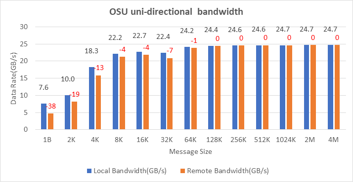 Figure 10: OSU Benchmark unidirectional bandwidth test on two servers with Intel 8380 processors and NVIDIA Mellanox HDR InfiniBand
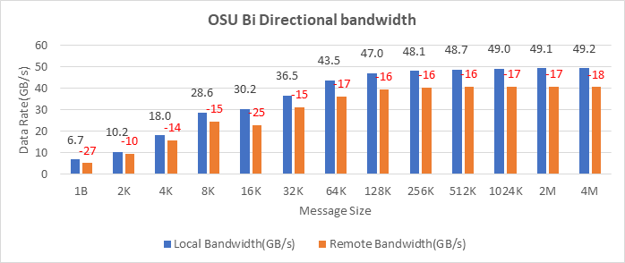 Figure 11: OSU Benchmark bi-directional bandwidth test on two servers with Intel 8380 processors and NVIDIA Mellanox HDR InfiniBand
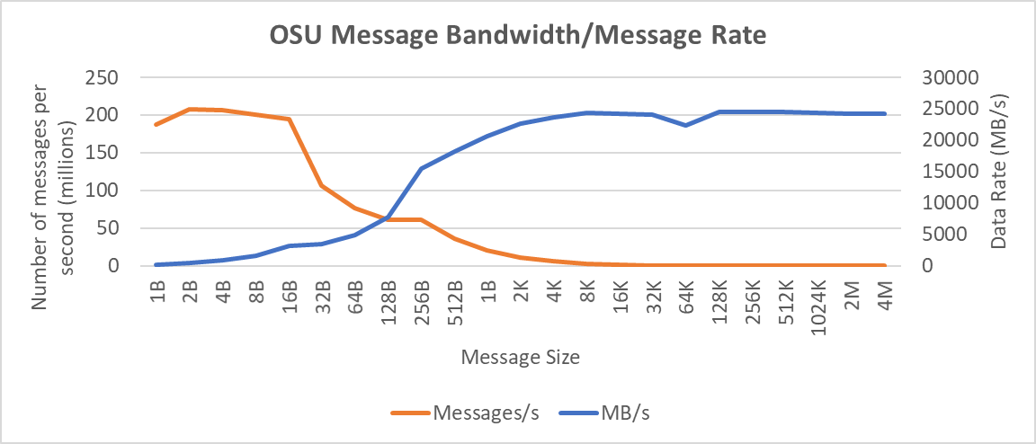
Figure 12: Interconnect bandwidth and message rate performance obtained between two servers having Intel 8380 processors with OSU Benchmark
On two nodes connected using the NVIDIA Mellanox ConnectX-6 HDR InfiniBand adapter cards, we achieved approximately 25 GB/s unidirectional bandwidth and a message rate of approximately 200 million messages/second—almost double the performance numbers obtained on the NVIDIA Mellanox HDR100 card.
Comparison with Cascade Lake processors
Based on the compute resources availability in our Dell EMC HPC & AI Innovation Lab, we selected the Cascade Lake processor-based servers and benchmarked them with software listed in Table 1. Figure 13 through Figure 16 show performance results from the Intel Ice Lake and Cascade Lake processors. The numbers over the bars represent the relative change in the application performance with respect to the application performance obtained on the Intel 6252 Cascade Lake processor.
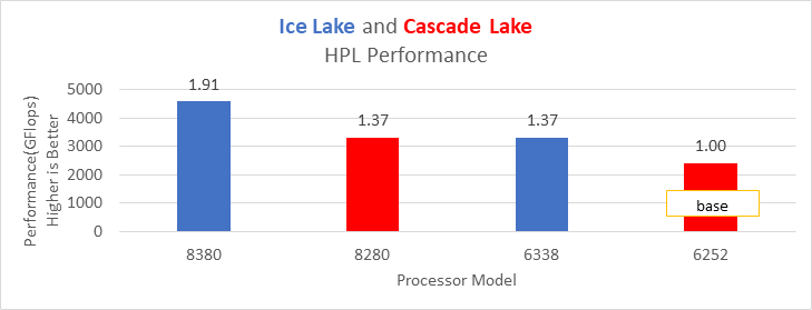 Figure 13: HPL performance on processors listed in Table 2
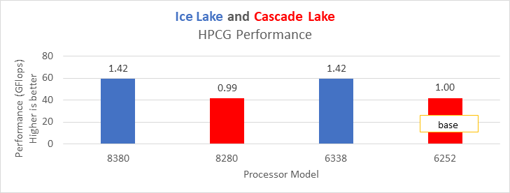 Figure 14: HPCG performance on processors listed in Table 2
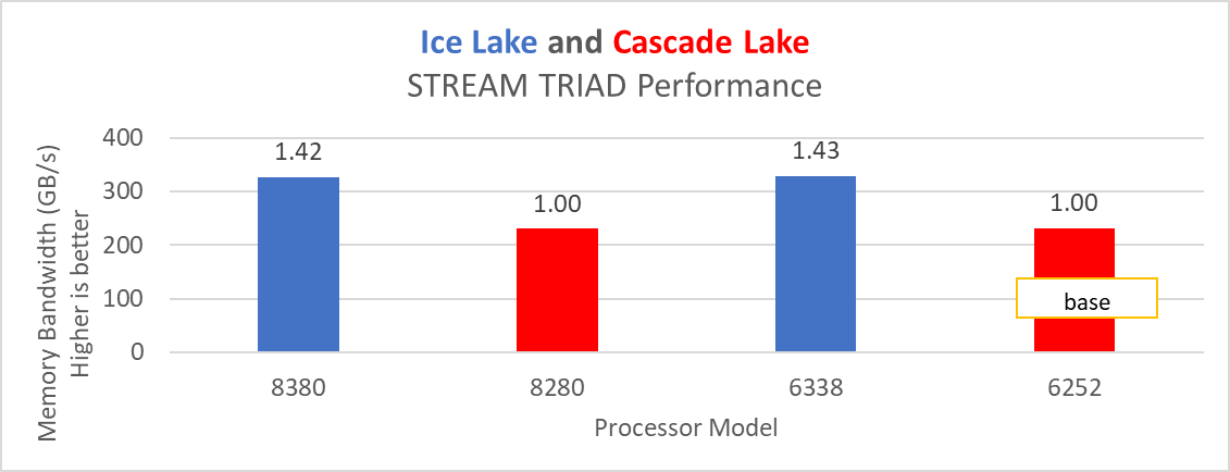 Figure 15: STREAM TRIAD test performance on Processors listed in Table 2
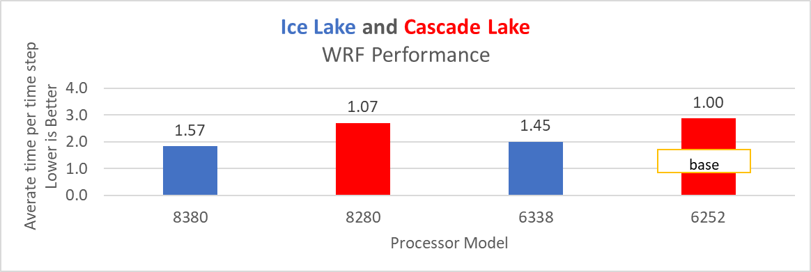 Figure 16: WRF performance on Processors listed in Table 2
Ice Lake delivers approximately 38 percent better performance than Cascade Lake with HPL on the top-end processor model. The memory bandwidth-bound benchmarks such as STREAM and HPCG (see Figure 13 and Figure 14) delivered 42 percent to 43 percent performance improvement over the top-end Cascade Lake processors addressed in this blog.
The average real-time power usage of the Dell EMC PowerEdge platforms (listed in Table 1) was measured with the synthetic benchmarks listed in this blog. Figure 17 compares the power usage data from the Cascade Lake and Ice Lake platforms. The number over the bar represents the relative change of power with respect to the base (Intel 6252 processor in the idle state) power measured.
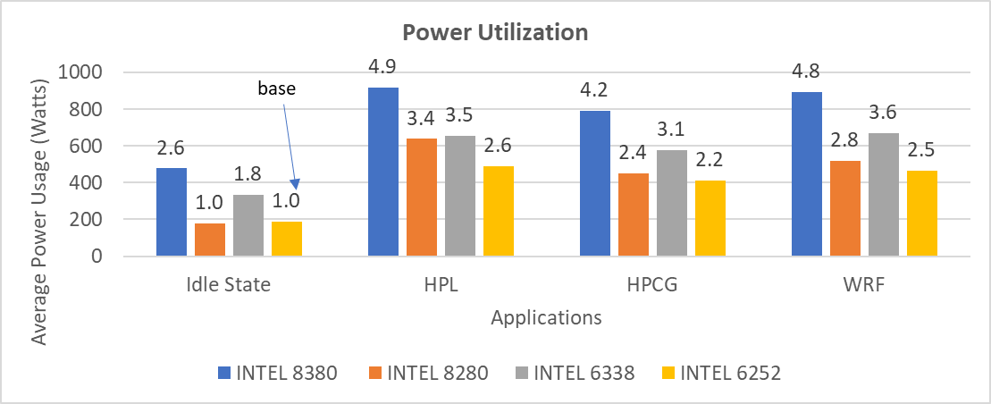
Figure 17: Average power usage during benchmark runs on Dell EMC PowerEdge servers (see details in Table 1)
Considering the data with the Performance Optimized profile with the respective power measurement, the applications (depending on the processor model) were unable to deliver better performance per watt on the Ice Lake platform when compared to the Cascade Lake platform.
Summary and future work
The Ice Lake processor-based Dell EMC Power Edge servers, with notable hardware feature upgrades over Cascade Lake, show up to 47 percent performance gain for all the HPC benchmarks addressed in this blog. Hyper-threading should be Disabled for the benchmarks addressed in this blog; for other workloads the option should be tested and enabled as appropriate. Watch this space for subsequent blogs that describe application performance studies on our new Ice Lake processor-based cluster.