The Demand Forecasting process consumes multiple business-specific datasets which produce the output weekly per demand signals. The streamlined workflows for these processes are described in Figure 2.

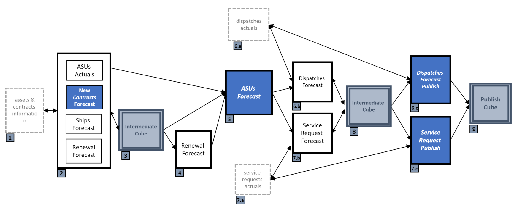
Figure 2.   Workflow diagram of forecasting process

Each workflow starts with contract forecast which is later reviewed and adjusted by business teams. ASUs, dispatches, and SRs forecasts are performed sequentially. The result is moved from SQL-server table and that later published into the cube for the end users’ consumption.  

Forecasting model development

Model working

The codes used to run the ARIMA timeseries forecasts are available as R scripts. ARIMA is a class of models that depends on timeseries and its own past values. In this process, eight different ARIMA model variants are used to forecast forward contracts, ASUs, and more. 

• Seasonal naive in which the last period's actuals are used as this period's forecast, without adjusting them or attempting to establish causal factors
• Fixed ARIMA:(0,0,1),(0,1,0)
• Fixed ARIMA:(0,1,2),(0,1,0)
• Fixed ARIMA:(1,0,0),(0,1,0)
• Fixed ARIMA:(1,1,1),(0,1,0)
• Exponential smooth a time series forecasting method for univariate data that can be extended to support data with a systematic trend or seasonal component.
• Auto exponential smooth (previously named forecast smoothing) is used to calculate optimal parameters of a set of smoothing functions
• Holt linear is forecasting method applies a triple exponential smoothing for level, trend and seasonal components

Out of these models, the one that minimizes the Root Mean Squared Error (RMSE) of the fit to a hold-out sample should be used in forecast result creation.

Each component in ARIMA functions as a parameter with a standard notation. For ARIMA models, a standard notation would be ARIMA with p, d, and q integers. In this model, integer values substitute for the parameters to indicate the type of ARIMA model used. The parameters can be defined as:

p: the number of lag observations in the model; also known as the lag order.

d: the number of times that the raw observations are differenced; also known as the degree of differencing.

q: the size of the moving average window; also known as the order of the moving average.

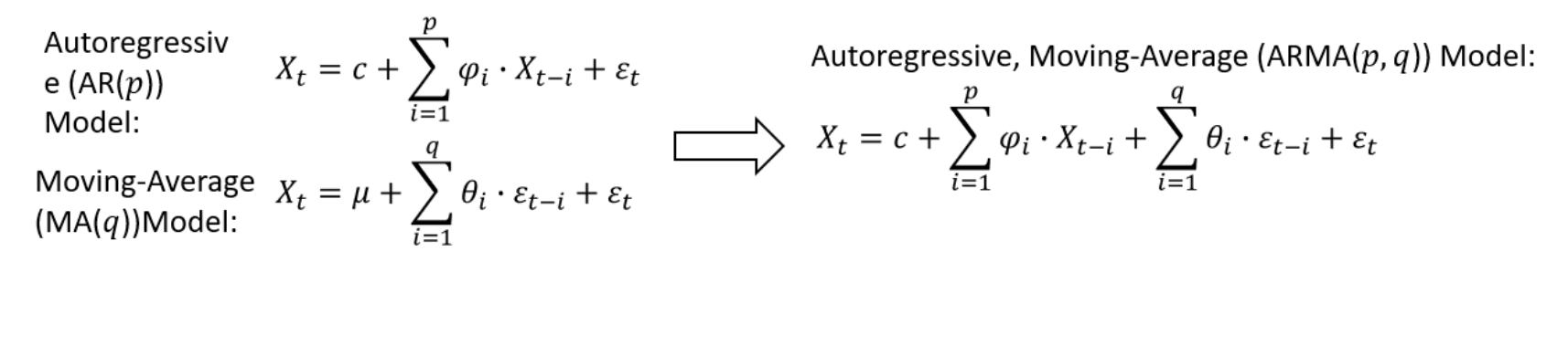In a linear regression model, for example, the number and type of terms are included. A 0 value, which can be used as a parameter, would mean that component should not be used in the model. This way, the ARIMA model can be constructed to perform the function of an ARIMA model, or even simple AR, I, or MA models.

In this model, p is the order of the Auto Regressive (AR) term. This term refers to the number of lags of X to be used as predictors and q is the order of the Moving Average (MA) term. It refers to the number of lagged forecast errors that should go into the ARIMA Model. 

The SRs and dispatches are forecast forward using the same ARIMA model variants that are used to forecast contract and ASUs.

SRs and dispatches are forecast forward on both count-basis and rate-basis methods. The forecast reported for each time series is selected based on the largest rate observed in the historical data; if the largest rate observed in the historical data is less than or equal to 0.005 (0.5 percent) the rate-based method is selected, but the count-based method is used if largest attach rate observed in the historical data is greater than 0.005.

The count-based method calculates the count of the forecast, whereas rate-based method calculates the rate by combining the count with the ASUs and forecasting. The rate method determines the forecast based on count volume per ASU basis. The rates used in this forecast include mean dispatch rate for dispatches (MDR) and inbound contact rate (ICR) for SRs.

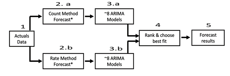
Figure 3.    Flowchart of model working

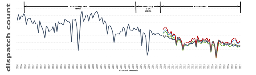
Figure 4.   Outcome of number of ARIMA timeseries models for dispatches counts w.r.t fiscal week

Some dispatches only occur during specific periods or once in a quarter and do not appear by statistical failures but by proactive customer engagement. Those dispatch forecasts are not generated using the ARIMA models, but it based on quarterly averages computed from the last four completed quarters. 

Model improvement methods

To improve the overall computation time and incorporate forecast disturbances, such as COVID-19 in demand signal forecasting, the following model improvement approaches are being used to reduce the manual dependency of choosing the hyperparameters. This means that parameters with values that control the learning process and determine the values of model parameters that a learning algorithm.

Low volume and high volume forecast

Analysis of low and high volume forecasts showed that running various forecasting models on a low volume timeseries does not have a significant impact in the accuracy of the outcome and only increases the runtime. Therefore, it is preferred to use one simple model for the low volume and running all different models on the high-volume timeseries. This setup not only provides better results, but also saves runtime. Using low volume data reduces computation time by 80 percent and improves accuracy by about 25 percent.

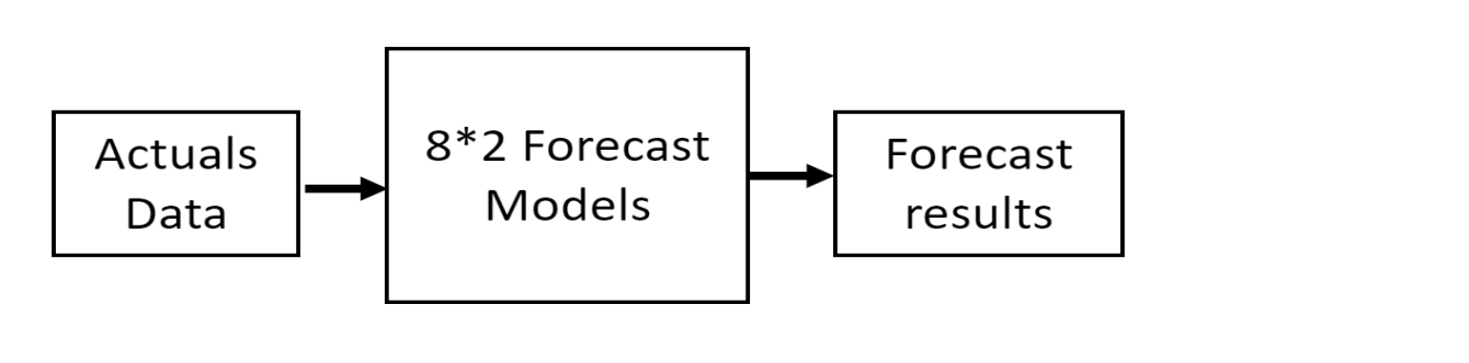
Figure 4.   Flowchart without implementation of High, Low and Zero volume methods

Figure 5.   Flowchart without implementation of High, Low, and Zero volume methods

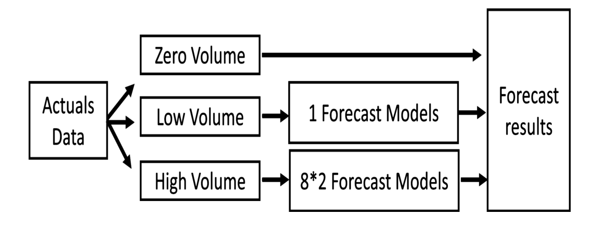
Figure 6.   Flowchart after implementation of high, low, and zero volume methods

COVID-19 normalization

A COVID-19 impact analysis showed businesses required a forecast that does not incorporate variations caused by COVID-19 to accurately predict future (post-COVID-19) forecasts. A forecast before COVID-19 was used to create a normalization/delta profile for each timeseries. This forecast normalized the COVID effect before the historical data was used for forecasting. The pre-COVID-19 forecast results were used as input data for producing future forecast results. Figure 5 shows COVID-19 based data (shown in blue) and forecast results of pre-COVID-19 (shown in orange). 

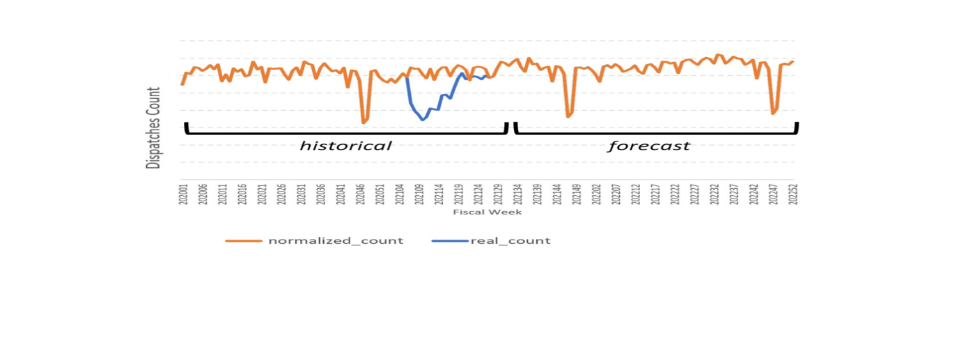
Figure 7.   COVID-19 normalization for dispatches counts w.r.t fiscal week

Holiday significance

Holiday significance analyses show large variations in count volume in all demand signals such as ASUs, SRs, and dispatches. The date of certain holidays can vary each year which in turn changes the date of the demand signal variations that occur each year. Initially, timeseries are created without including holidays as a feature component. Relevant holidays provided by businesses are used as external regressors to produce the final timeseries which incorporate the effect of holidays in each timeseries.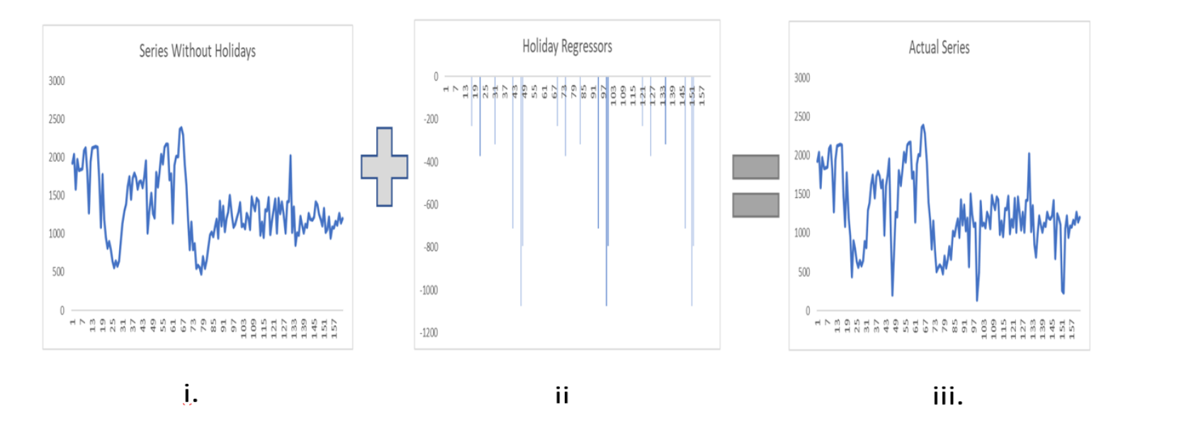 

Figure 8.   Representation of pre and post timeseries after including holiday regressors

Discontinuity detection and correction

Data quality and other factors negatively impact the quality of the forecast and cause significant shifts and discontinuities in historical data. Problematic timeseries are detected by dividing the timeseries into several segments and checking the variations of the counts. Drastic variations are likely caused by discontinuity in the timeseries. These discontinuities can be autocorrected by using normalization methods to feed corrected data into the forecast model.

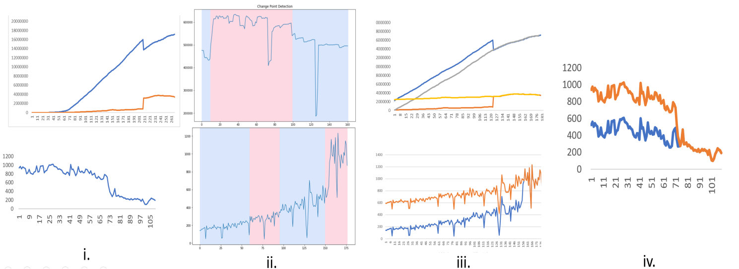
Figure 9.   Representation of problematic discontinuous data and auto correcting it with cleaned data

• 9i shows discontinuity in timeseries. 
• 9ii detects the point where the discrepancy occurs in the timeseries.
• 9iii shows correction or feeding clean data to make the timeseries smooth. 
• 9iv shows the final output timeseries.  

Dynamic threshold settings

Dynamic threshold settings are driven by an ML model that creates threshold for each timeseries dynamically based on accuracy of the method (such as rate based and count based.)

Classification and clustering techniques are used to understand which set of time series should use count-based and which set should use the rate-based model, depending on the accuracy of the forecast. Classification using the Random Forest, LightGBM, and CatBoost classifier approaches from which CatBoost has accurate precision (60 percent) and recall (80 percent) results.

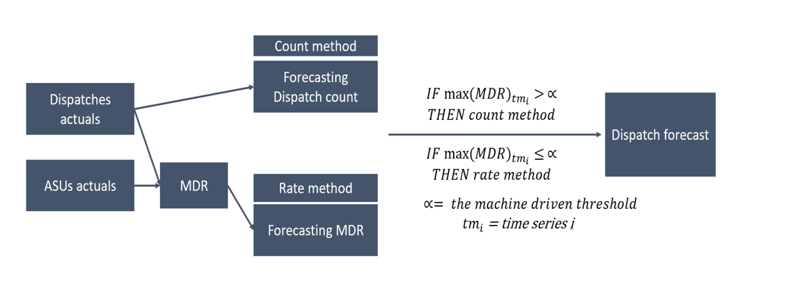
Figure 10.   Process to identify the threshold value (α) which helps choose the best method

Results and discussion

The demand forecasting of all signals including ASUs, contract, renewals, dispatches, and SRs are based on each product’s availability in each segment is conducted based on real data. These results are analyzed to inform future forecasts. This study examines the effectiveness of each timeseries. The final results are displayed in the following graphs.

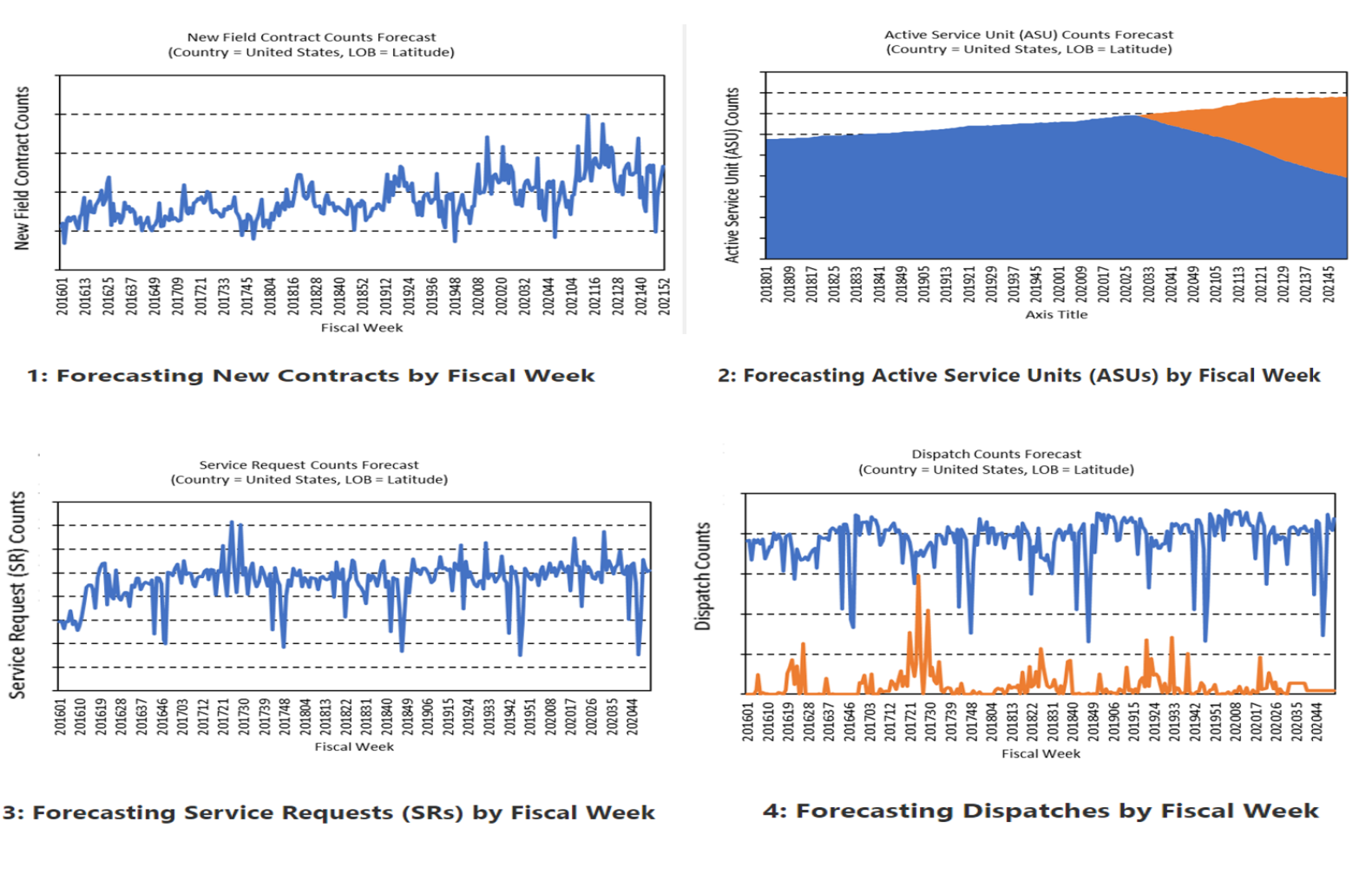 Figure 11.    Final forecast results for all demand signals 

We used many forecast model evaluation metrics to evaluate the model accuracy, such as:

• Mean error (ME): ME - average of all the errors in a set
• Mean absolute error (MAE): MAE - absolute values of errors
• Mean percent error (MPE): MPE - average of percentage errors by which forecasts of a model differ from actual values of the quantity being forecast
• Mean absolute percent error (MAPE): MAPE - average of the absolute percentage errors of forecasts
• Mean absolute squared error (MASE): MASE- mean absolute error of the forecast values, divided by the mean absolute error
• RMSE: the model selected is the one that minimizes the RMSE of the fit to a hold-out sample that conveys the standard deviation of the residuals, meaning it describes the concentration of the data

The final forecast reported for each LOB is the one that fits the time series the best over the last quarter.

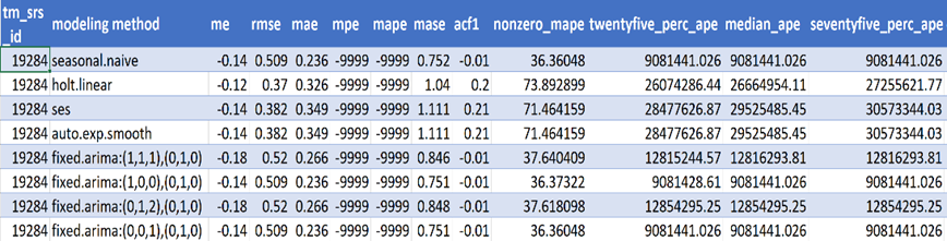
Figure 12.    Evaluation matrix of timeseries based on single unique-id assigned to each timeseries