Imagine this scenario: You are a data scientist on the data science team at a large company, and your team is trying to build a character recognition model that performs well on the famous MNIST dataset. The MNIST dataset is a collection of scanned images with hand-drawn integers, from 0-9. Your team is going to train a computer vision model that can accurately predict new handwritten numbers based on the information contained within each image of the MNIST data. 

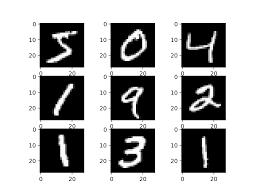
Example MNIST scanned images

This task is part of a larger initiative for your company: an application that can convert human-written pages into computer-readable text. Your team’s model will provide a key part of the number-recognition functionality of this application. Accuracy is important, and your manager, Yoshua, has tasked your team with developing a model that achieves 97.5 percent accuracy on unseen samples (your holdout or test set). 

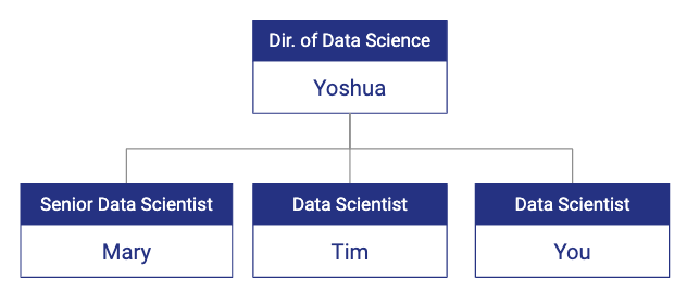
Your data science team organizational chart

Project Framework

This isn’t the first project your team has worked on together, so you already have a useful project framework. Traditionally, your team defines the steps of a modeling process in the following way:

1. Problem identification
2. Data wrangling
3. Preprocessing and training data development
4. Modeling (which often loops back to any step 1-4)
5. Documentation

In this case, steps 1and 2 have already been completed because you’re working with MNIST, a well-known, clean dataset with a good balance of samples for each number 0-9.

[1] Problem Identification

Correctly classify numbers in images of hand-drawn integers from 0 to 9.

[2] Data Wrangling

You will use the MNIST dataset to train your model. This is a research-grade dataset, so you and your team do not need to invest time in assembling, labeling, cleaning and storing a dataset for this modeling task.

Your team can move ahead with MNIST data into the exploratory data analysis (EDA) phase of your project. 

[3] Preprocessing and Training Data Development

While excellent results have been achieved with the MNIST data in the past without feature engineering prior to training, your team would nevertheless like to explore whether applying certain preprocessing methods will deliver a higher-accuracy model or faster time to convergence.

Data Modification 1: Remove constant 0- or 255-value pixels

To start, you decide you’d like to check whether there are any pixels that are background (black) in every dataset sample. If there are, you might try dropping those pixels, thereby reducing the size of the input data and potentially speeding up model training. 

Your intuition is correct! Some pixels always have an intensity of 0 (max = 0) or of 255 (min = 255). Since the pixels that always have an intensity of 255 (white) are members of the pixel groups that comprise the digits, you’ll leave those as is, but you remove all of the border (max = 0) pixels and create a new zero-pixel-removed dataset.

Data Modification 2: Normalize pixel values between 0 and 1 instead of between 0 and 255

Your colleague Mary has another good idea: normalizing the pixel values down from the original 0-255 scale to 0-1. Given that the model weights will be initialized randomly to values close to zero, it could take a long time for the weights to update sufficiently to manipulate input features on an orders-of-magnitude different scale. 

Normalizing the pixel values between 0 and 1 may help the models train faster. Mary completes this work and stores the dataset as a second preprocessed version of the baseline dataset.

For now, you and the team are satisfied with these two engineered datasets and the baseline dataset to start the modeling phase. If your models do not perform at or above the accuracy target, your team may return to this stage and explore other feature engineering and preprocessing techniques. 

[4] Modeling

The team now has three training datasets:

• Baseline MNIST
• Zero-pixel-removed MNIST
• Normalized MNIST

Your data science team is ready to start experimenting with modeling techniques. You’d like to try many different architectures and model families to find out what works best. The team comes up with a preliminary list to experiment with:

• MLP Neural Networks
• ConvNets
• ResNets
• Tree-based models

You, Mary and Tim decide to break up the work into three buckets. You each own one of the datasets (baseline, zero-pixel-removed and normalized). To get complete coverage of the modeling options, you will each own testing all four model types with your assigned dataset.

Your team decides that Comet is the right platform given the size of the team, number of experiments and short project timeline. You need to make sure every experiment is logged to one central dashboard every time you, Mary or Tim run a script or execute cells in a Jupyter notebook. That way, you can share insights, create custom visualizations and iterate more quickly toward a production-grade model. Yoshua also wants to use Comet so he can have visibility into how each approach is developing and who is working on what.

You are assigned the zero-value-pixel dataset. You developed good template code for ConvNets, ResNets, simple feedforward Neural Networks and XGBoost, so you quickly spin up some experiments. After logging into Comet, you go to your dashboard to see some results.

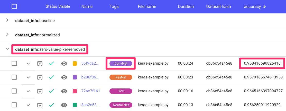
Comet Project UI

Right away, you can tell that your ConvNet models are outperforming the others, but you’re still not at the 97.5 percent accuracy your manager wants for this project. You quickly put together a couple of project-level visualizations to further inspect the performance of your models. 

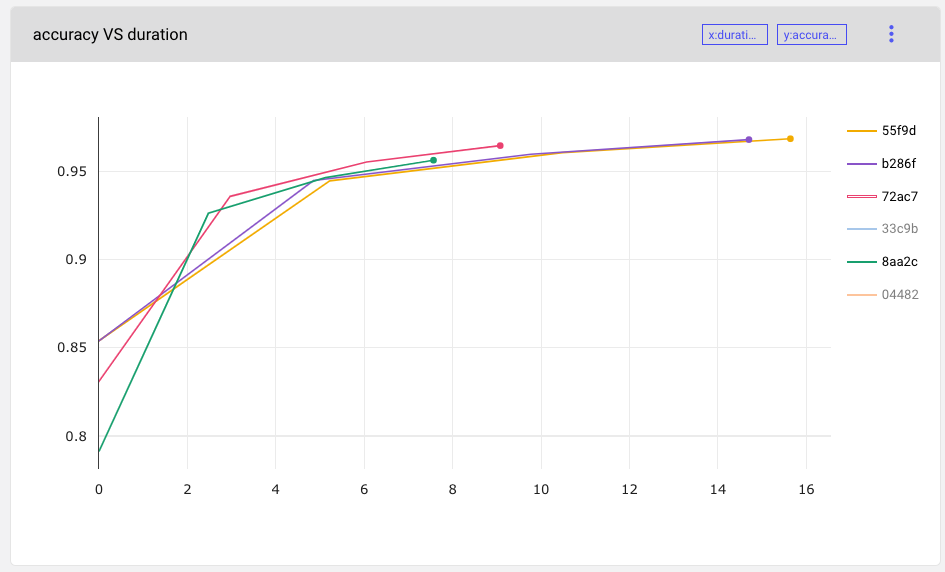
First, you’d like to compare accuracy across all experiments for your entire team, so you create a visualization charting model accuracy over time (duration of training).

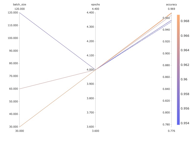
Next, you’d like a way to visualize the underlying hyperparameter space for each of your models. Comet provides a parallel coordinates template that gives you exactly what you need for now. The parallel coordinates view is simple, but you’ll add more hyperparameters later. Already, you can tell that lower batch sizes are outperforming larger ones. 

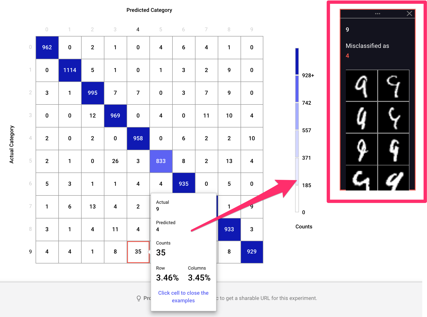
You decide to inspect your CNN model in more detail by spinning up a confusion matrix to identify common misclassifications. Comet’s built-in module for this does the trick and lets you inspect each box to see specific samples that are being misclassified. 

While you analyze your first batch of experiments, you see new ones popping up in Comet. Your teammates are also at work. By using Comet, you can immediately compare experiments that you’re each contributing to in one central workspace. 

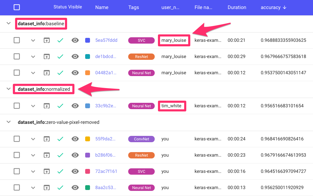
Once your team has completed baseline models with a fixed set of hyperparameters for each architecture for each dataset, you sit down together and make some decisions about where to focus next. It seems that, from the first pass, the zero-value-pixel-removed dataset is yielding slightly higher-accuracy models, given identical architectures and hyperparameter settings. 

As one last sanity check, you select the two best experiments trained on the zero-value-pixel-removed dataset and use the Comet “Diff” feature to compare every aspect of each experiment.

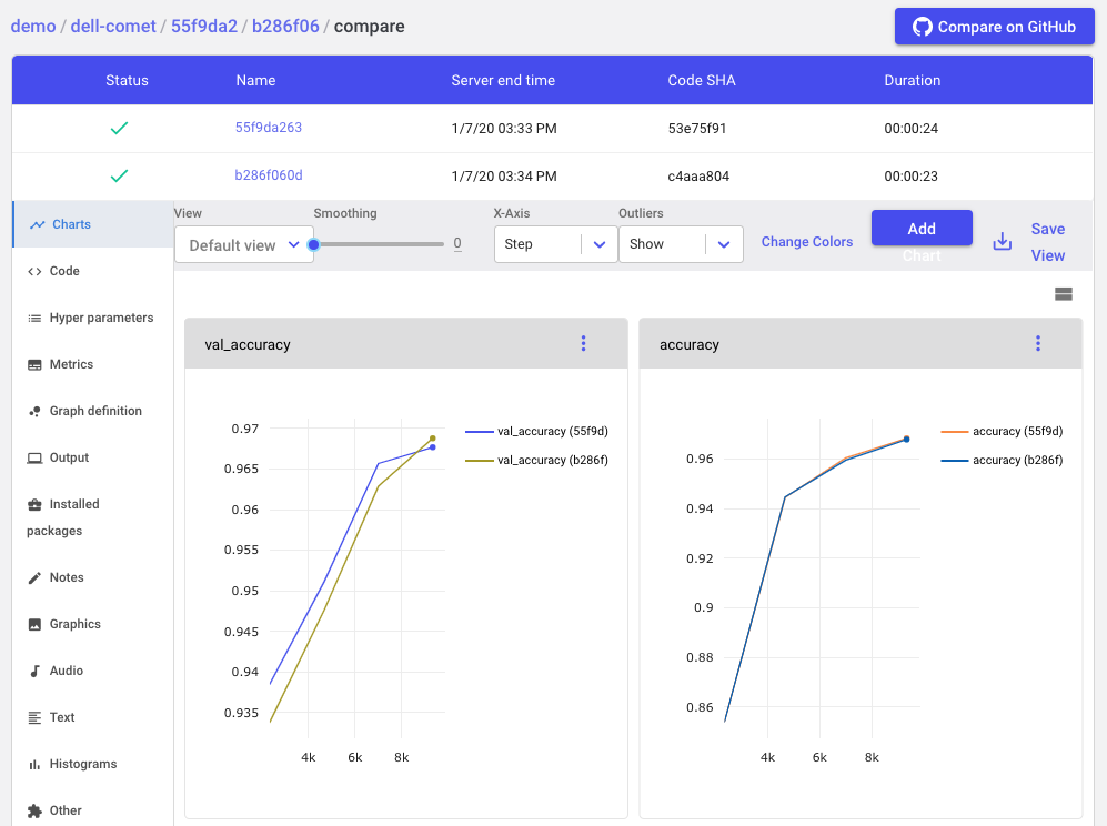
The Comet “Diff” feature allows data scientists to compare everything about two experiments: metrics, code, hyperparameters, dependencies, system information and more, right in the UI.

Well aware that parameter tuning may cause this to change, you decide to focus on the zero-pixel-removed dataset for the next stage of research, taking your best performing architecture and conducting a hyperparameter optimization to try and identify a set of hyperparameters that will yield better results.

One day, Yoshua pulls you and Mary aside and asks if you’d be willing to assist another data science pod for a short two-week project, putting your MNIST classifier work on hold. They’re working on the character recognition model for alphabet letters and have hit a roadblock. You and Mary agree to have Tim run the next phase of your research project — the optimization — while you and Mary spend a couple of weeks assisting the other team.

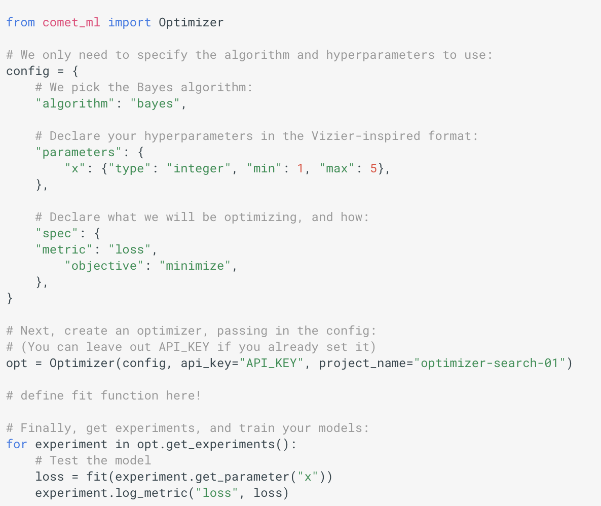
Comet’s built-in Optimizer allows Tim to do the experimentation efficiently and without spending too much time setting up testing code and managing the sweep.

After completing the sweep, Tim inspects the performance of each experiment visually to look for insights. Right away something interesting jumps out at him: models where kernel size equals 5 are almost always outperforming other models. 

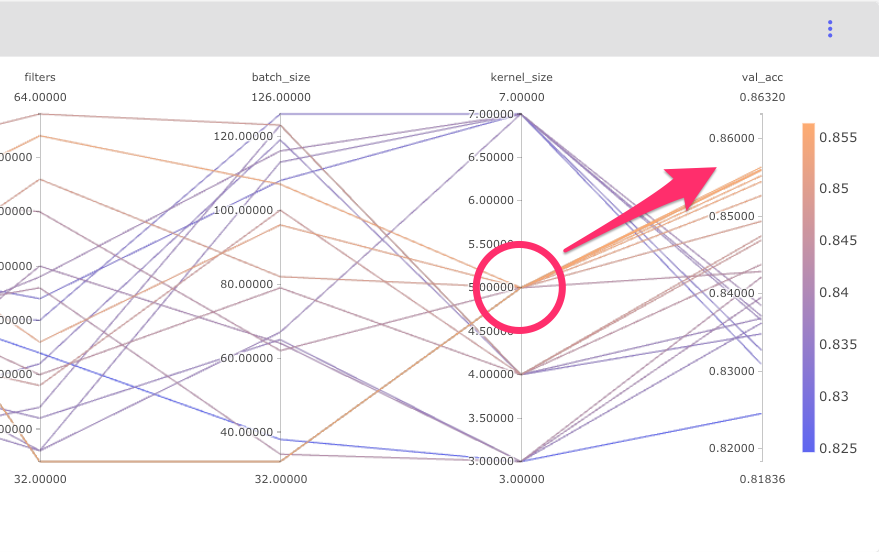
Comet Parallel Coordinates Chart

Armed with these new insights, the whole team is ready to sit down and plan the next steps. Now that you and Mary are back from assisting the other team, you quickly see that the best model is right around 97.5 percent accuracy on test data — exactly where your manager wanted you to be! You can either keep digging on the convolutional network, zero-pixel-removed data combination or dive into other combinations. 

It comes as a huge surprise when, the next Monday, Tim lets your boss know that he is leaving the company. Not only is Tim a huge asset to your team, but he has also built up a ton of modeling intuition for this MNIST project and ran the entire hyperparameter optimization phase of your research cycle solo. 

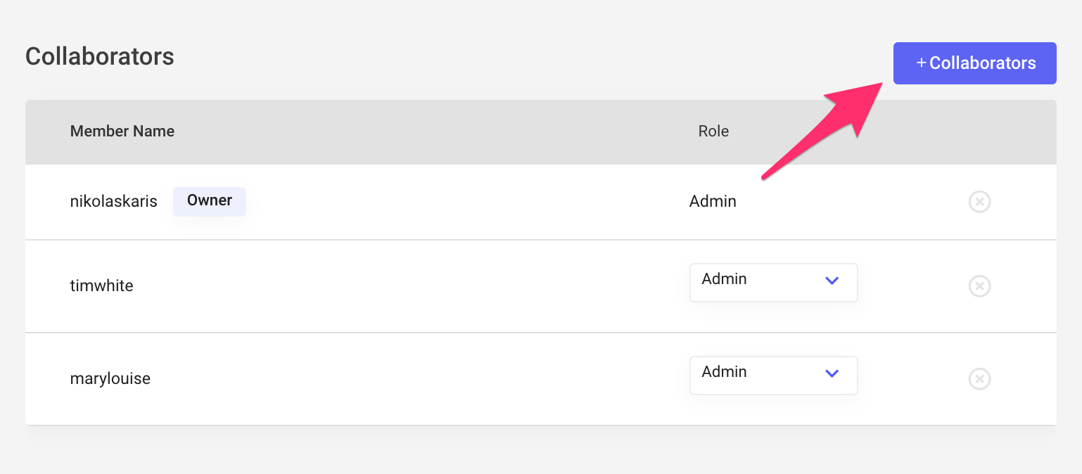
Thankfully, your team had a few Ph.D. interns over the past year, so you’re quickly able to make a replacement hire. And, again, the decision to use Comet saves a ton of effort as your new data scientist, Sara, gets up and running in a fraction of the time it would have taken her without access to this system of record. 

[6] Documentation

Because your team adopted Comet, you get great documentation for free! All of the modeling decisions, experimentation history, performance, and team-wide record keeping have all been taken care of for you. You get to spend more time on the activities that add value to the team and the company.

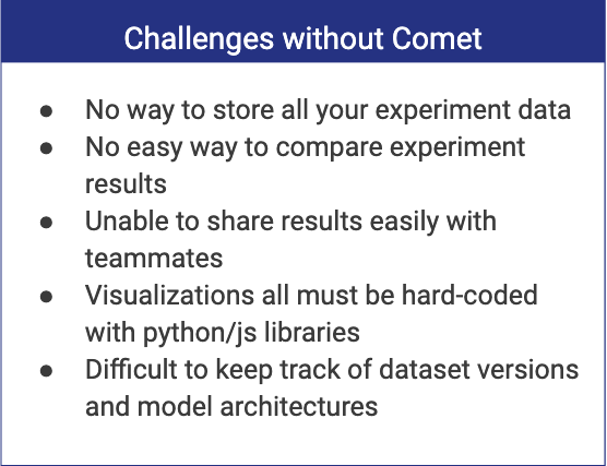
Conclusion

This user story highlights some of the common challenges for data science teams during a typical modeling project. Comet provides a solution to many of these challenges, and can allow any data science team, large or small, to work more collaboratively, transparently and with faster research cycles. The partnership between Dell EMC and Comet ensures that using Comet with Dell EMC’s AI-enabled infrastructure stacks is the shortest path to improved productivity for any organization.