
Performance evaluation of BWA-GATK pipelines
Performance evaluation of BWA-GATK pipelines
-
Test case 1: BWA-GATK v3.6
This pipeline is designed to perform germline variant calling. The performances of the pipeline are measured in runtime (hours) and genomes per day.
Single sample performance
A single sample (50x WGS) is processed with 6248, 8352Y, and 8358, and the results are shown in Figure 6. The runtime with 8352Y decreased by 10% from 6348 while 8358 runs 11% faster.
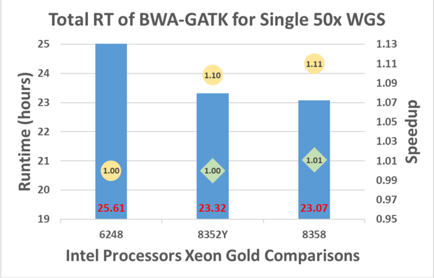
Figure 6. BWA-GATK v3.6 performance with single-sample and single-node
Note: Circles represent the speedups of 8352Y and 8358 from 6248 whereas diamonds represent 8358’s speedup from 8352Y.
Throughput of single node: multisample and single-node performance
As the number of samples processed concurrently increased (x-axis in Figure 7), the runtime to complete multiple pipelines increased (left y-axis in Figure 7). With 14 samples processed on a single compute node in 49.86 hours, genomes per day are calculated to be 6.74 (right y-axis in Figure 7). This capacity is the maximum for a single C6520 with an Intel 8358 CPU.
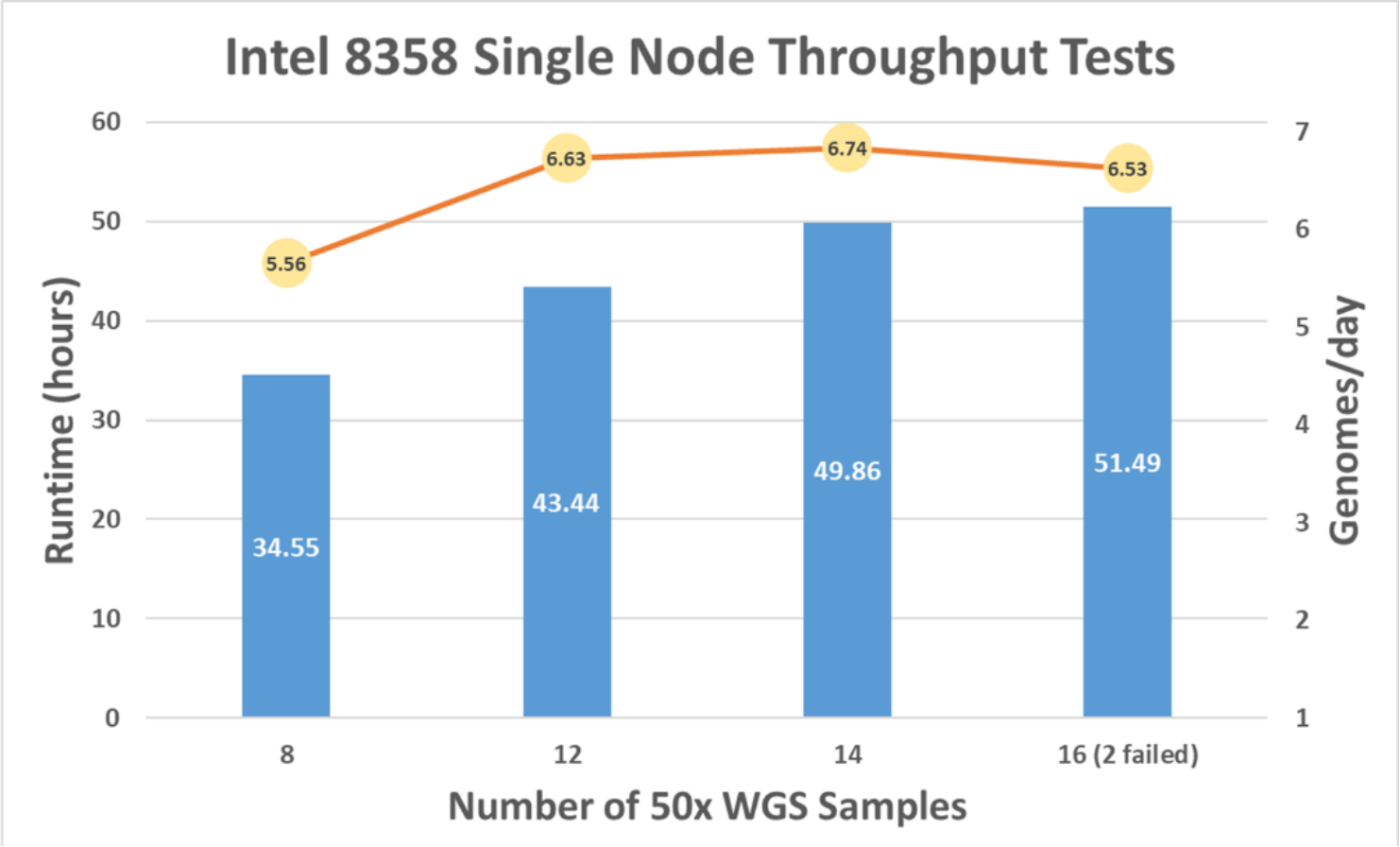
Figure 7. BWA-GATK v3.6 performance with multisample and single-node
Throughput of multiple nodes: multisample and multinode performance
From the multisample and single-node performance study, 14 samples per C6520 is the maximum number of samples that can be processed together. However, the number of samples per C6520 is set to 12 to avoid any failures.
Figure 8 shows the runtime and genomes/day metrics for the performance of the pipeline. There are some runtime variations along with two, four, and eight compute node tests since the test environment was not isolated for this study. Network and storage congestions can interfere with the tests at any given time. The more C6520s used, the number of genomes per day increases exponentially, and there is no sign of network and storage problems with 32 C6520s and 384 50x WGS samples. It is verifiable that the system can handle 384 50x WGS in 46.84 hours (196.75 genomes/day).
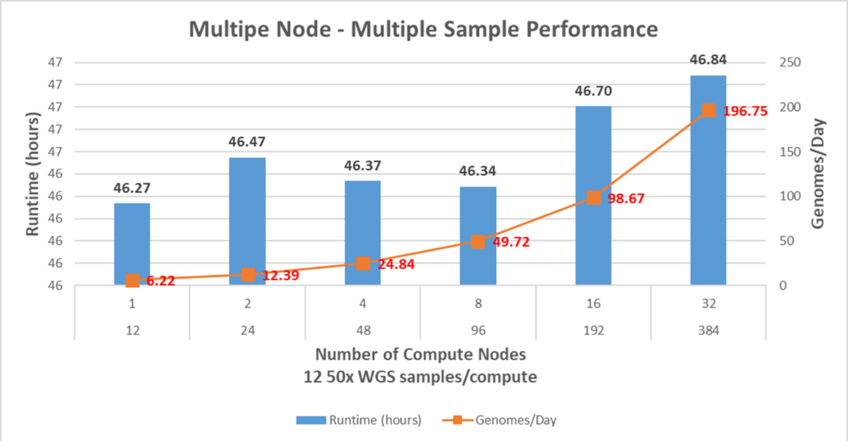
Figure 8. BWA-GATK v3.6 performance with multisample and multinode performance
Test Case 2: BWA-GATK v4.2 without data parallelization
The runtime of each step in the BWA-GATK v4.2 pipeline is shown in Table 9.
As GATK steps are limited to using a single core, especially the runtime for the variant calling step increases to about 29 hours from about seven hours. Even if the genomes per day metric can be increased by processing more samples together, the throughput from this version of the pipeline will not improve meaningfully.
Table 9. BWA-GATK v4.2 performance without data parallelization
Step
Operation
Cores
Runtime (hours)
1
Align and Sort
64
2.73
2
Mark and Remove Duplicates
64
4.92
3
Recalibrate Base and Generate BQSR
1
6.56
4
Apply BQSR
1
4.32
5
Call Variants
1
29.22
6
Consolidate GVCFs
1
0.31
Total Runtime
48.06
Genomes/day
0.50
Test case 3: BWA-GATK v4.2 with data parallelization
First, 50x WGS is split into 64 chunks at the DP 1 step. Each chunk of input sequence reads is aligned and removed duplicates in Steps 1 and 2 with a single core. The outcome from Step 2 is 64 BAM files. These BAM files are merged into a single BAM file in the order of chromosome locations. These two additional steps added 1.73 hours, but the runtime reduction on Steps 1 and 2 is around10 hours. Also, the data can be parallelized easily after the DP2 step without diluting statistical power, if the data is split into multiple chunks in the order of chromosome locations.
Instead of splitting the merged BAM file physically, a series of index files are created at DP 4 step. A total of 64 interval files were created, and each interval file contains a consecutive chromosomal region pointing to an equal number of sequence reads to minimize runtime variations.
DP 5 is another additional step that combines all results (VCF chunks) from Step 6 into a single VCF. This step can be an option since each VCF is fully functional.
The total runtime with this new pipeline is 5.50 hours, and it can process 4.36 genomes per day.
It is worth noting that the level of data parallelization in the pipeline depends on the network and storage bandwidths. The pipeline read from a set of two input files and generated 64 chunks of each. The size of input files used for the test was around 110 GB in gzip compressed format. And the size of each chunk was slightly less than 1 GB in gzip format. Hence, the storage system needs to write 128 1GB files simultaneously. If storage does not have enough bandwidth to handle many files concurrently, the storage will handle the chunks one at a time. This situation will increase runtime even more than without data parallelization.
It is recommended that a preliminary study to find out what is the optimal number of splits (the level of data parallelization) before adopting this type of data parallelization.
Table 10. BWA-GATK v4.2 performance with data parallelization
Step
Operation
Number of Splits
Cores
Runtime (hours)
DP 1
Split FASTQ file
64
64
1.38
1
Align and Sort
64
1
1.28
2
Mark and Remove Duplicates
64
1
0.19
DP 2
Merge BAM files
1
1
0.35
DP 3
Count the number of aligned reads
1
1
0.04
DP 4
Generate Interval files
64
1
0.45
3
Recalibrate Base and Generate BQSR
64
1
0.12
4
Apply BQSR
64
1
0.16
5
Call Variants
64
1
1.04
6
Consolidate GVCFs
64
1
0.01
DP 5
Merge VCF files
1
1
0.49
Total Runtime
5.50
Genomes/day
4.36