


Training an AI Radiologist with Distributed Deep Learning
Wed, 07 Dec 2022 13:25:02 -0000
|Read Time: 0 minutes
Originally published on Aug 16, 2018 11:14:00 AM
The potential of neural networks to transform healthcare is evident. From image classification to dictation and translation, neural networks are achieving or exceeding human capabilities. And they are only getting better at these tasks as the quantity of data increases.
But there’s another way in which neural networks can potentially transform the healthcare industry: Knowledge can be replicated at virtually no cost. Take radiology as an example: To train 100 radiologists, you must teach each individual person the skills necessary to identify diseases in x-ray images of patients’ bodies. To make 100 AI-enabled radiologist assistants, you take the neural network model you trained to read x-ray images and load it into 100 different devices.
The hurdle is training the model. It takes a large amount of cleaned, curated, labeled data to train an image classification model. Once you’ve prepared the training data, it can take days, weeks, or even months to train a neural network. Even once you’ve trained a neural network model, it might not be smart enough to perform the desired task. So, you try again. And again. Eventually, you will train a model that passes the test and can be used out in the world.
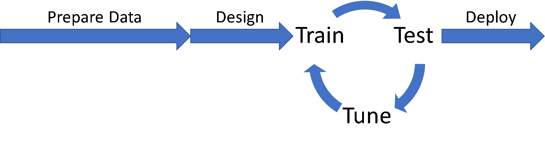 Workflow for developing neural network modelsIn this post, I’m going to talk about how to reduce the time spent in the Train/Test/Tune cycle by speeding up the training portion with distributed deep learning, using a test case we developed in Dell EMC’s HPC & AI Innovation Lab to classify pathologies in chest x-ray images. Through a combination of distributed deep learning, optimizer selection, and neural network topology selection, we were able to not only speed the process of training models from days to minutes, we were also able to improve the classification accuracy significantly.
Starting Point: Stanford University’s CheXNet
We began by surveying the landscape of AI projects in healthcare, and Andrew Ng’s group at Stanford University provided our starting point. CheXNet was a project to demonstrate a neural network’s ability to accurately classify cases of pneumonia in chest x-ray images.
The dataset that Stanford used was ChestXray14, which was developed and made available by the United States’ National Institutes of Health (NIH). The dataset contains over 120,000 images of frontal chest x-rays, each potentially labeled with one or more of fourteen different thoracic pathologies. The data set is very unbalanced, with more than half of the data set images having no listed pathologies.
Stanford decided to use DenseNet, a neural network topology which had just been announced as the Best Paper at the 2017 Conference on Computer Vision and Pattern Recognition (CVPR), to solve the problem. The DenseNet topology is a deep network of repeating blocks over convolutions linked with residual connections. Blocks end with a batch normalization, followed by some additional convolution and pooling to link the blocks. At the end of the network, a fully connected layer is used to perform the classification.
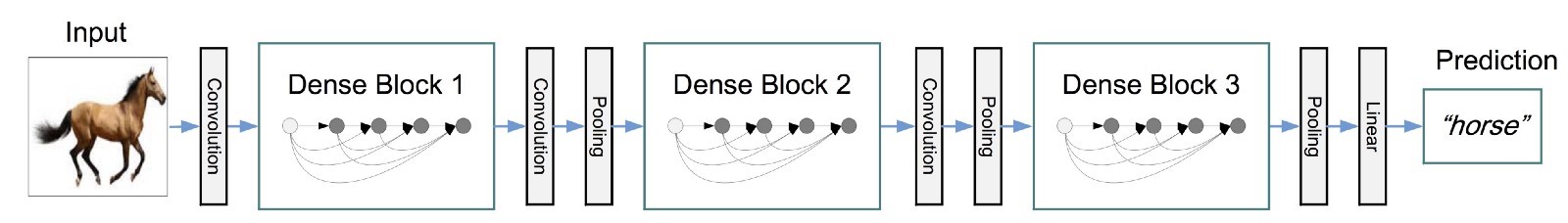 An illustration of the DenseNet topology (source: Kaggle)
Stanford’s team used a DenseNet topology with the layer weights pretrained on ImageNet and replaced the original ImageNet classification layer with a new fully connected layer of 14 neurons, one for each pathology in the ChestXray14 dataset.
Building CheXNet in Keras
It’s sounds like it would be difficult to setup. Thankfully, Keras (provided with TensorFlow) provides a simple, straightforward way of taking standard neural network topologies and bolting-on new classification layers.
from tensorflow import keras
from keras.applications import DenseNet121

orig_net = DenseNet121(include_top=False, weights='imagenet', input_shape=(256,256,3))
In this code snippet, we are importing the original DenseNet neural network (DenseNet121) and removing the classification layer with the include_top=False argument. We also automatically import the pretrained ImageNet weights and set the image size to 256x256, with 3 channels (red, green, blue).
With the original network imported, we can begin to construct the classification layer. If you look at the illustration of DenseNet above, you will notice that the classification layer is preceded by a pooling layer. We can add this pooling layer back to the new network with a single Keras function call, and we can call the resulting topology the neural network's filters, or the part of the neural network which extracts all the key features used for classification.
from keras.layers import GlobalAveragePooling2D

filters = GlobalAveragePooling2D()(orig_net.output)
The next task is to define the classification layer. The ChestXray14 dataset has 14 labeled pathologies, so we have one neuron for each label. We also activate each neuron with the sigmoid activation function, and use the output of the feature filter portion of our network as the input to the classifiers.
from keras.layers import Dense

classifiers = Dense(14, activation='sigmoid', bias_initializer='ones')(filters)
The choice of sigmoid as an activation function is due to the multi-label nature of the data set. For problems where only one label ever applies to a given image (e.g., dog, cat, sandwich), a softmax activation would be preferable. In the case of ChestXray14, images can show signs of multiple pathologies, and the model should rightfully identify high probabilities for multiple classifications when appropriate.
Finally, we can put the feature filters and the classifiers together to create a single, trainable model.
from keras.models import Model

chexnet = Model(inputs=orig_net.inputs, outputs=classifiers)
With the final model configuration in place, the model can then be compiled and trained.
Accelerating the Train/Test/Tune Cycle with Distributed Deep Learning
To produce better models sooner, we need to accelerate the Train/Test/Tune cycle. Because testing and tuning are mostly sequential, training is the best place to look for potential optimization.
How exactly do we speed up the training process? In Accelerating Insights with Distributed Deep Learning, Michael Bennett and I discuss the three ways in which deep learning can be accelerated by distributing work and parallelizing the process:
- Parameter server models such as in Caffe or distributed TensorFlow,
- Ring-AllReduce approaches such as Uber’s Horovod, and
- Hybrid approaches for Hadoop/Spark environments such as Intel BigDL.
Which approach you pick depends on your deep learning framework of choice and the compute environment that you will be using. For the tests described here we performed the training in house on the Zenith supercomputer in the Dell EMC HPC & AI Innovation Lab. The ring-allreduce approach enabled by Uber’s Horovod framework made the most sense for taking advantage of a system tuned for HPC workloads, and which takes advantage of Intel Omni-Path (OPA) networking for fast inter-node communication. The ring-allreduce approach would also be appropriate for solutions such as the Dell EMC Ready Solutions for AI, Deep Learning with NVIDIA.
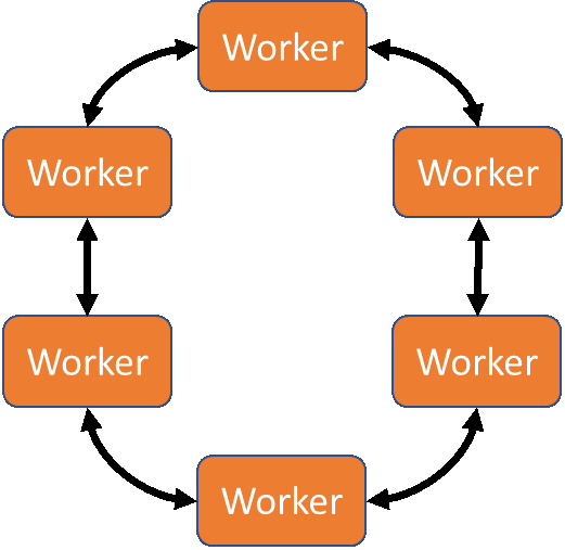 The MPI-RingAllreduce approach to distributed deep learning
Horovod is an MPI-based framework for performing reduction operations between identical copies of the otherwise sequential training script. Because it is MPI-based, you will need to be sure that an MPI compiler (mpicc) is available in the working environment before installing horovod.
Adding Horovod to a Keras-defined Model
Adding Horovod to any Keras-defined neural network model only requires a few code modifications:
- Initializing the MPI environment,
- Broadcasting initial random weights or checkpoint weights to all workers,
- Wrapping the optimizer function to enable multi-node gradient summation,
- Average metrics among workers, and
- Limiting checkpoint writing to a single worker.
Horovod also provides helper functions and callbacks for optional capabilities that are useful when performing distributed deep learning, such as learning-rate warmup/decay and metric averaging.
Initializing the MPI Environment
Initializing the MPI environment in Horovod only requires calling the init method:
import horovod.keras as hvd

hvd.init()
This will ensure that the MPI_Init function is called, setting up the communications structure and assigning ranks to all workers.
Broadcasting Weights
Broadcasting the neuron weights is done using a callback to the Model.fit Keras method. In fact, many of Horovod’s features are implemented as callbacks to Model.fit, so it’s worthwhile to define a callback list object for holding all the callbacks.
callbacks = [ hvd.callbacks.BroadcastGlobalVariablesCallback(0) ]
You’ll notice that the BroadcastGlobalVariablesCallback takes a single argument that’s been set to 0. This is the root worker, which will be responsible for reading checkpoint files or generating new initial weights, broadcasting weights at the beginning of the training run, and writing checkpoint files periodically so that work is not lost if a training job fails or terminates.
Wrapping the Optimizer Function
The optimizer function must be wrapped so that it can aggregate error information from all workers before executing. Horovod’s DistributedOptimizer function can wrap any optimizer which inherits Keras’ base Optimizer class, including SGD, Adam, Adadelta, Adagrad, and others.
import keras.optimizers

opt = hvd.DistributedOptimizer(keras.optimizers.Adadelta(lr=1.0))
The distributed optimizer will now use the MPI_Allgather collective to aggregate error information from training batches onto all workers, rather than collecting them only to the root worker. This allows the workers to independently update their models rather than waiting for the root to re-broadcast updated weights before beginning the next training batch.
Averaging Metrics
Between steps error metrics need to be averaged to calculate global loss. Horovod provides another callback function to do this called MetricAverageCallback.
callbacks = [ hvd.callbacks.BroadcastGlobalVariablesCallback(0),
              hvd.callbacks.MetricAverageCallback()
            ]
This will ensure that optimizations are performed on the global metrics, not the metrics local to each worker.
Writing Checkpoints from a Single Worker
When using distributed deep learning, it’s important that only one worker write checkpoint files to ensure that multiple workers writing to the same file does not produce a race condition, which could lead to checkpoint corruption.
Checkpoint writing in Keras is enabled by another callback to Model.fit. However, we only want to call this callback from one worker instead of all workers. By convention, we use worker 0 for this task, but technically we could use any worker for this task. The one good thing about worker 0 is that even if you decide to run your distributed deep learning job with only 1 worker, that worker will be worker 0.
callbacks = [ ... ]

if hvd.rank() == 0:
 callbacks.append(keras.callbacks.ModelCheckpoint('./checkpoint-{epoch].h5'))
Result: A Smarter Model, Faster!
Once a neural network can be trained in a distributed fashion across multiple workers, the Train/Test/Tune cycle can be sped up dramatically.
The figure below shows exactly how dramatically. The three tests shown are the training speed of the Keras DenseNet model on a single Zenith node without distributed deep learning (far left), the Keras DenseNet model with distributed deep learning on 32 Zenith nodes (64 MPI processes, 2 MPI processes per node, center), and a Keras VGG16 version using distributed deep learning on 64 Zenith nodes (128 MPI processes, 2 MPI processes per node, far right). By using 32 nodes instead of a single node, distributed deep learning was able to provide a 47x improvement in training speed, taking the training time for 10 epochs on the ChestXray14 data set from 2 days (50 hours) to less than 2 hours!
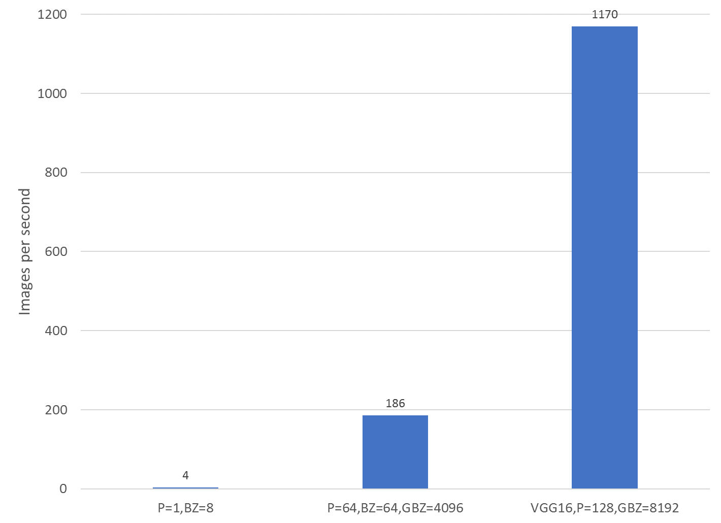 Performance comparisons of Keras models with distributed deep learning using Horovod
The VGG variant, trained on 128 Zenith nodes, was able to complete the same number of epochs as was required for the single-node DenseNet version to train in less than an hour, although it required more epochs to train. It also, however, was able to converge to a higher-quality solution. This VGG-based model outperformed the baseline, single-node model in 4 of 14 conditions, and was able to achieve nearly 90% accuracy in classifying emphysema.
 Accuracy comparison of baseline single-node DenseNet model vs VGG variant with Horovod
Conclusion
In this post we’ve shown you how to accelerate the Train/Test/Tune cycle when developing neural network-based models by speeding up the training phase with distributed deep learning. We walked through the process of transforming a Keras-based model to take advantage of multiple nodes using the Horovod framework, and how these few simple code changes, coupled with some additional compute infrastructure, can reduce the time needed to train a model from days to minutes, allowing more time for the testing and tuning pieces of the cycle. More time for tuning means higher-quality models, which means better outcomes for patients, customers, or whomever will benefit from the deployment of your model.
Lucas A. Wilson, Ph.D. is the Chief Data Scientist in Dell EMC's HPC & AI Innovation Lab. (Twitter: @lucasawilson)